
2. Return values, macros, programs#
Let’s briefly recap what we covered last week and what you’ve practiced this week in lab:
Importing data
We’ll be managing datafiles both locally and remotely
In the Basic class all file management is local, but syntax for importing remote files is considered
The Advanced class will be Unix based, and Stata is but one of the statistical packages you’ll be considering
Performing basic queries
Mostly covered in the Basic class
Outputing some of your findings into .xlsx, .log, etc.
Here we’ll go beyond the Basic class’ focus on .log & .xlsx as output files Today we’ll build on these ideas:
String values as output
Lets consider the data from the week one survey
Numeric values embedded within a string
Using
macros
Examples beyond .xlsx and .log
Show code cell source
import networkx as nx
import matplotlib.pyplot as plt
#import numpy as np
#import sklearn as skl
#

#plt.figure(figsize=[2, 2])
G = nx.DiGraph()
G.add_node("user",  pos = (550,500) )
G.add_node("system",  pos = (-550,500) )
G.add_node("program",  pos = (-2000, 960) )
G.add_node("syntax",  pos = (2000, 950) )
G.add_node("ado", pos = (-3000, 550) )
G.add_node("do", pos = (3000, 550) )
G.add_node("command", pos = (-1900, 150) )
G.add_node("queue", pos = (1900, 150) )
G.add_node("results", pos = (0,0))
G.add_node("dta", pos = (0, -475))
G.add_node("log", pos = (-1900, -475))
G.add_node("excel", pos = (-4000, -475))
G.add_node("word", pos = (1900, -475))
G.add_node("html", pos = (4000, -475))
G.add_node("publish", pos = (0, -950))
G.add_edges_from([ ("program","ado"), ("syntax", "do")])
G.add_edges_from([("ado", "command"), ("do", "queue") ])
G.add_edges_from([("command", "results"), ("queue", "results"),("results","excel"),("results","word"),("results","html")])
G.add_edges_from([("results","dta"),("results","log")])
G.add_edges_from([("dta","publish"),("log","publish"),("excel","publish"),("word","publish"),("html","publish")])
nx.draw(G,
        nx.get_node_attributes(G, 'pos'),
        with_labels=True,
        font_weight='bold',
        node_size = 4500,
        node_color = "lightblue",
        linewidths = 3)
ax= plt.gca()
ax.collections[0].set_edgecolor("#000000")
ax.set_xlim([-5000, 5000])
ax.set_ylim([-1000, 1000])
plt.show()
2.0 Case-study#
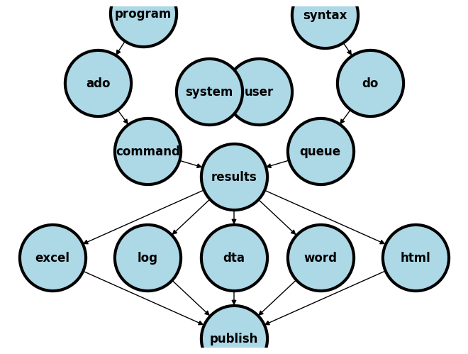
A sequence or queue of instructions
commands + syntax = codegiven to Stata via a do-file will generate resultsNever include results in your do-file when you share your work in this class and with future collaborators
Due diligence in the
open-scienceenterprise demands that othersreproduceyour results and findingsYour duty is to share only the
input, and ours is to reproduce youroutputso as to fullfil our shared CredoPlease share your do-files and any third-party ado-files, if at all your script or do-file relies on third-party programs
HTML & LaTeX#
.xlsx
.log
.dta
.docx
-
Self-publication
GitHub-Pages
Macros embedded in output
2.1 xlsx#
Instructions for Data Analysis and Report Generation#
2.1.1 Preparation#
Setting the Working Directory: Begin by defining some macros. In this case, we define a global macro
$path, whose value is a specified directory, which will serve as the primary workspace for the project. Edit this path to suit your workdirectory.
global path "/users/d/desktop"
cd $path
Simulation of Dataset: Execute the Stata do-file located at the provided URL to simulate the dataset necessary for the analysis (from hw1).
qui do https://raw.githubusercontent.com/jhustata/hw1/main/simulation.do
2.1.2 Data Analysis and Report Generation#
Directory for Week 3: Create a new directory within the working environment to organize the outputs related to this week’s analysis.
mkdir wk3
Initialization of Excel File for Table 1: Set up an Excel file within the newly created directory to prepare for the output of Table 1, which will detail the demographic characteristics of the participants in the main safety population.
putexcel set wk3/Table1
putexcel A1="Table 1. Demographic Characteristics of the Participants in the Main Safety Population"
Inspection of Working Directory Contents: Utilize the list command to view the contents of the working directory, ensuring that all necessary files are present and correctly organized.
ls -l
2.1.3 Composition of Table 1 using your own code#
Column 1 (Characteristics):
Label the characteristics column, followed by the specific demographic detail to be analyzed (in this case, Female - no. (%)).
putexcel A2=("Characteristics")
putexcel A3=("Female - no. (%)")
Column 2 (BNT162 Group Analysis):
Execute a series of commands to calculate and display the number of participants in the trial arm (BNT162), as well as the number and percentage of female participants within this group.
ds

// trial arm
sum bnt if bnt==1
local bnt_1: di r(N)
di `bnt_1'

// women in trial arm
sum female if female==1 & bnt==1
local bnt_1_fN: di r(N)
di `bnt_1_fN'

// as a percentage of total population
local bnt_1_fper=`bnt_1_fN'*100/`bnt_1' //arithmetic & macros; equal sign
di `bnt_1_fper'
local bnt_1_fper: di %3.1f `bnt_1_fper' //formatting & macros; `: di` syntax
di `bnt_1_fper'
Output to Excel:
Format and export the calculated data to the designated Excel file, ensuring accurate representation of the demographic characteristics under investigation.
putexcel B1=("BNT162")
putexcel B2=("N=`bnt_1'")
putexcel B3=("`bnt_1_fN' (`bnt_1_fper')")
Questions:
Can you now populate the adjacent cells for the placebo arm?
How about populating rows for all kinds of variables
Binary (e.g. female)
Continuous (e.g. age)
Categorical (e.g. country)
2.2 log#
Let’s input some Stata code into your .do file
log using chi2.log, replace //creates a .log file
use transplants, clear //imports the datafile
tab dx gender, row  chi2 //performs a chi-square test
log close //closes the .log file
Now lets find the content of the .log file created. When analyzing data in Stata, one often encounters the need to review or share results in a format that is both informative and easily interpretable. An essential step in this process involves examining the output stored in log-files. These files capture the essence of your analytical work, including statistical tests and their results. A common feature of interest in these results is the p-value, a metric that helps us understand the significance of our findings.
. tab dx gender, row  chi2

+----------------+
Key
------------------
frequency
row percentage
+----------------+

Primary            gender
Diagnosis      |    0    |    1	    | Total
---------------+---------+----------+------
1=Glomerular   |  237    |    187   |	 424
               |  55.90  |   44.10  | 100.00
---------------+---------+----------+------
2=Diabetes     | 60      |  37	    | 97
               | 61.86   |  38.14   | 100.00
---------------+---------+----------+------
3=PKD          | 81      |  66	    | 147
               | 55.10   |  44.90   | 100.00
---------------+---------+----------+------
4=Hypertensive | 316     |  176	    | 492
               | 64.23   |  35.77   | 100.00
---------------+---------+----------+------
5=Renovascular | 24      |  15	    | 39
               | 61.54   |  38.46   | 100.00
---------------+---------+----------+------
6=Congenital   | 46      |  22	    | 68
               | 67.65   |  32.35   | 100.00
---------------+---------+----------+------
7=Tubulo       | 32      |  35	    | 67
               | 47.76   |  52.24   | 100.00
---------------+---------+----------+------
8=Neoplasm     | 8       |  5	    | 13
               | 61.54   |  38.46   | 100.00
---------------+---------+----------+------
9=Other        | 421     |  232	    | 653
               | 64.47   |  35.53   | 100.00
---------------+---------+----------+------
Total          | 1,225   |  775     | 2,000
               | 61.25   |  38.75   | 100.00

Pearson chi2(8) =  18.4805	Pr	= 0.018

.
To start, let’s consider the return list command:
return list
This command is your gateway to reviewing the most recent test results stored by Stata. It lists out all the statistics calculated by the last command, including the number of observations (r(N)), test statistics like chi-squared values (r(chi2)), and crucially, the p-value (r(p)).
However, simply listing out the p-value isn’t always enough, especially when preparing your findings for a broader audience, such as in peer-reviewed publications. The reporting of p-values follows specific conventions to enhance clarity and understanding. Let’s explore how to apply these conventions using a conditional formatting approach:
2.2.1 Introduction to the “quietly” Command#
The first block introduces the concept of running commands ‘quietly’ in Stata, which suppresses the output in the Results window.
qui {
    // Your Stata commands here
}
qui {: This command is short for ‘quietly’. It tells Stata to execute the commands within the braces without displaying the usual output in the Results window. It’s helpful for keeping your results clean or when you’re only interested in the final outcome rather than seeing every step.}: This closing brace marks the end of the ‘quietly’ section. After this point, Stata will return to its default behavior, which is to display output for each command.
2.2.2 Handling p-values Less Than 0.01#
The second block explains how to handle cases where p-values are less than 0.01.
qui {
    if r(p) < 0.01 {
        local p: di "p < 0.01"
    }
}
if r(p) < 0.01 {: This line checks if the p-value (r(p)) from the last statistical test is less than 0.01. If true, the commands inside the braces will execute.local p: di "p < 0.01": Here, if the condition is met, we assign a formatted string “p < 0.01” to a local macro namedp. This is a concise way to communicate that the test results are highly significant.
2.2.3 Formatting p-values Between 0.01 and 0.05#
The third block focuses on p-values that fall between 0.01 and 0.05, using precision formatting.
qui {
    else if inrange(r(p),0.01,0.05) {
        local p: di %3.2f r(p)
    }
}
else if inrange(r(p),0.01,0.05) {: This line checks if the p-value is within the specified range. Theinrange()function is versatile, allowing for clear boundary definitions.local p: di %3.2f r(p): For p-values in this range, we format the number to have two decimal places (e.g., 0.03), ensuring clarity and precision in our reporting.
2.2.4 Formatting p-values Greater Than 0.05#
The fourth block deals with formatting p-values greater than 0.05.
qui {
    else {
        local p: di %2.1f r(p)
    }
}
else {: This part catches any cases not previously covered, essentially p-values greater than 0.05.local p: di %2.1f r(p): Here, we format the p-value to have one decimal place, indicating a less strict interpretation of statistical significance.
2.2.5 Combining Everything#
Finally, we combine all the parts into a cohesive whole, demonstrating how to format p-values based on their value, all within a ‘quietly’ block.
qui { //asks Stata to work "quietly", until the corresponding brace is closed at the end
    if r(p) < 0.01 {
       local p: di "p < 0.01"
    }
    else if inrange(r(p),0.01,0.05) {
       local p: di %3.2f r(p)
    }
    else {
       local p: di %2.1f r(p)
    }
    noi di "p = `p'"
} //after this brace Stata may return to its default: "noisely" produce output as it runs the program
This final block puts everything together, showing how to use
quito suppress unnecessary output while precisely formatting p-values according to their significance level. Thenoi di "p =p’`” line then displays the formatted p-value, completing the explanation of how to communicate statistical results clearly and effectively.
2.2.6 Recap of the chi-square test#
In this script, we start by checking if the p-value is less than 0.01. If so, we report it as “p < 0.01” to indicate a very high level of statistical significance. This convention signals to the reader that the result is significant beyond the conventional thresholds.
If the p-value falls between 0.01 and 0.05, we report it in a standard numeric format (e.g., 0.03), maintaining two decimal places for precision. This range indicates statistical significance at the conventional 5% level, which is widely accepted in many research disciplines.
For p-values greater than 0.05, we format them with one decimal place, acknowledging that while the result may not meet the conventional threshold for statistical significance, it is still worth reporting for a comprehensive understanding of the analysis.
This approach to formatting and reporting p-values is not just about following academic conventions; it’s about making your results clear and interpretable for your audience, facilitating better understanding and discussion of your research findings.
In practice, here’s how the output might look after applying our formatting script:
. return list

scalars:
r(N) =  2000
r(r) =  9
r(c) =  2
r(chi2) =  18.48047641017726
r(p) =  .0178990677414798

. qui {
p = 0.02
Notice how the p-value is processed and reported as “0.02” to fit the specified format for p-values between 0.01 and 0.05. This precision in reporting underscores the importance of statistical details in the broader narrative of your research findings.
2.3 dta#
Step 1: Clearing the Workspace
cls
clear
postutil clear
cls: Clears the Stata command window, providing a clean slate for your next commands. It’s a good practice to start with this to avoid confusion from previous outputs.clear: Removes all data from memory. This ensures that the workspace is clean before starting new data manipulations.postutil clear: Clears any existing posted datasets from memory. This is particularly useful when you’re about to create new posted datasets, ensuring no conflicts or errors arise from previous sessions.
Step 2: Setting Up a New Posted File
postfile pp str80 a float(b c) using output.dta, replace
postfile pp str80 a float(b c) using output.dta, replace: This line initiates the creation of a new dataset (output.dta) with specific variablesa,b, andc. Here,ppis the name given to this posting session,str80 adefinesaas a string variable with a maximum length of 80 characters, andfloat(b c)definesbandcas floating-point numbers. Thereplaceoption allows overwriting any existing file with the same name, ensuring that your new data is saved without issues.
Step 3: Populating the Dataset
post pp ("1") (24.4) (123)
post pp ("2") (31.5) (164)
post pp ("3") (29.0) (118)
These lines use the
postcommand to add records to the dataset you’ve started. Eachpostcommand adds a new row with the specified values fora,b, andc. For example,post pp ("1") (24.4) (123)adds a row withaas “1”,bas 24.4, andcas 123.
Step 4: Finalizing the Dataset
postclose pp
postclose pp: This command closes the posting session namedpp, finalizing the dataset. After this, no more data can be added tooutput.dtaunder this posting session.
Step 5: Using and Viewing the Dataset
use output, clear
list
use output, clear: Loads the newly createdoutput.dtainto memory, clearing any other data that was previously loaded. This makesoutput.dtathe active dataset for analysis.list: Displays the contents of the active dataset in the Results window. This provides a quick way to review the data you’ve just posted, ensuring it looks as expected.
2.4 docx#
We may embed Stata results in a .docx file in two very distinct ways:
putdocx
dyndoc
2.4.1. Putdocx#
putdocx begin (Tell Stata you want to create a Word doc)
putdocx text etc. (Define the contents of the Word doc you will create)
putdocx save (Actually create the Word doc and write it to disk)
putdocx clear
putdocx begin
putdocx paragraph
putdocx text ("How to embed Stata results in .docx")
putdocx paragraph
putdocx text ("Author, MD MPH")
putdocx paragraph
putdocx text ("Background. A user downloads and installs a system of program files, mostly ado-files, which form the foundation of most of the commands used in Stata Programming. Using those commands and additional syntax written out sequentially in a do-file, the user creates well-formed instruction to Stata called a do-file script. Once the user runs this script, results are generated and displayed in the results window, in a graph, or in a format (.xlsx, .log, .dta, .docx, .md, LaTeX, .html, etc). The .docx file format is of specific interest to us right now. To illustrate how this may be achieved in Stata, we hereby introduce the putdocx command.")
putdocx paragraph
putdocx text ("Methods. We created a do-file and populated it with this abstract using plain text. Results that might be numeric, string, alphanumeric, or formatted as macros are manually embeded in the text. We then saved this document using the file extension .do; however, any text file extension will work (.txt, .md, .do, etc). In the key analysis, Y = b0 + b1X, where Y is life expectancy at birth in years, the outcome or dependent variable; X is the country, the predictor or independent variable being tested.")
putdocx paragraph
putdocx text ("Results. We identified the newly created .html file in our folder and opened it to compare its format to this markdown file. And we saw all that we had made, and behold, it was very good. Ghastly macros in the original markdown language now appeared as neatly formatted results. There were 68 observations and 6 observations in the analyzed dataset. Average life expectancy of all countries, b0, was 72 years. Difference in life expectancy among adjacent countries, b1, showed no trend or pattern and was 0.002 year, essentially zero, and p=0.95")
putdocx paragraph
putdocx text ("Conclusion. In walking you through syntax, do-file creation, queued commands, generated results, through to embedding neatly formatted output in .html, we believe you now have a solid sense of all that Stata has to offer you. These ideas can be generalized to embedding results in .xlsx, .log, .dta, .docx, etc.")
putdocx save myfirst.docx, replace
Author, MD MPH
Background. A user downloads and installs a system of program files, mostly ado-files, which form the foundation of most of the commands used in Stata Programming. Using those commands and additional syntax written out sequentially in a do-file, the user creates well-formed instruction to Stata called a do- file script. Once the user runs this script, results are generated and displayed in the results window, in a graph, or in a format (.xlsx, .log, .dta, .docx, .md, LaTeX, .html, etc). The .docx file format is of specific interest to us right now. To illustrate how this may be achieved in Stata, we hereby introduce the putdocx command.
Methods. We created a do-file and populated it with this abstract using plain text. Results that might be numeric, string, alphanumeric, or formatted as macros are manually embeded in the text. We then saved this document using the file extension .do; however, any text file extension will work (.txt, .md, .do, etc). In the key analysis, Y = b0 + b1X, where Y is life expectancy at birth in years, the outcome or dependent variable; X is the country, the predictor or independent variable being tested.
Results. We identified the newly created .html file in our folder and opened it to compare its format to this markdown file. And we saw all that we had made, and behold, it was very good. Ghastly macros in the original markdown language now appeared as neatly formatted results. There were 68 observations and 6 observations in the analyzed dataset. Average life expectancy of all countries, b0, was 72 years. Difference in life expectancy among adjacent countries, b1, showed no trend or pattern and was 0.002 year, essentially zero, and p=0.95
Conclusion. In walking you through syntax, do-file creation, queued commands, generated results, through to embedding neatly formatted output in .html, we believe you now have a solid sense of all that Stata has to offer you. These ideas can be generalized to embedding results in .xlsx, .log, .dta, .docx, etc.
2.4.2. dyndoc#
Identical to the .html approach discussed in the next section
But has some caveats that we will discuss
Word documents are not able to render LaTeX format
Author, MD MPH#
Background:
A user downloads and installs a system of program files, mostly ado-files, which form the foundation of most of the commands
used in Stata Programming. Using those commands and additional syntax written out sequentially in a do-file, the user creates
well-formed instruction to Stata called a do-file script. Once the user runs this script, results are generated and displayed
in the results window, in a graph, or in a format (.xlsx, .log, .dta, .docx, .md, LaTeX, .html, etc). The .docx file format is of specific
interest since its the one of the most widely used word processors. To illustrate how this may be achieved in Stata, we hereby introduce the dyndoc
command.
Methods:
We created a do-file and populated it with this abstract using markdown language. Anything
in this document that is not ordinary text including <<dd_version: 2>>, <<dd_do:nooutput>>, <</dd_do>>, <<dd_display: c(N)>> is a
markup.
Results that might be numeric, string, alphanumeric, or formatted as macros are embeded at these markedup points. We then saved this
document using the file extension .do; however, any text file extension will work (.txt, .md, .do, etc). To the pwd where we saved
this text file, we added a cascading style sheet stmarkdown.css and header.txt to enhance the aesthetic of our .html file. Finally, we typed the
following command into the Stata command window: dyndoc filename.do, saving(filename.docx) replace. In the key analysis, \(Y = \beta_0 + \beta_1 X\), where \(Y\) is life expectancy at birth in years, the outcome or dependent variable; \(X\) is the country, the predictor or independent variable being tested.
. webuse lifeexp, clear
(Life expectancy, 1998)
. encode country, gen(Country)
. quietly sum lexp
. qui local lexp_mean: di %3.0f r(mean)
. quietly sum Country
. qui local Country_mean: di r(mean)
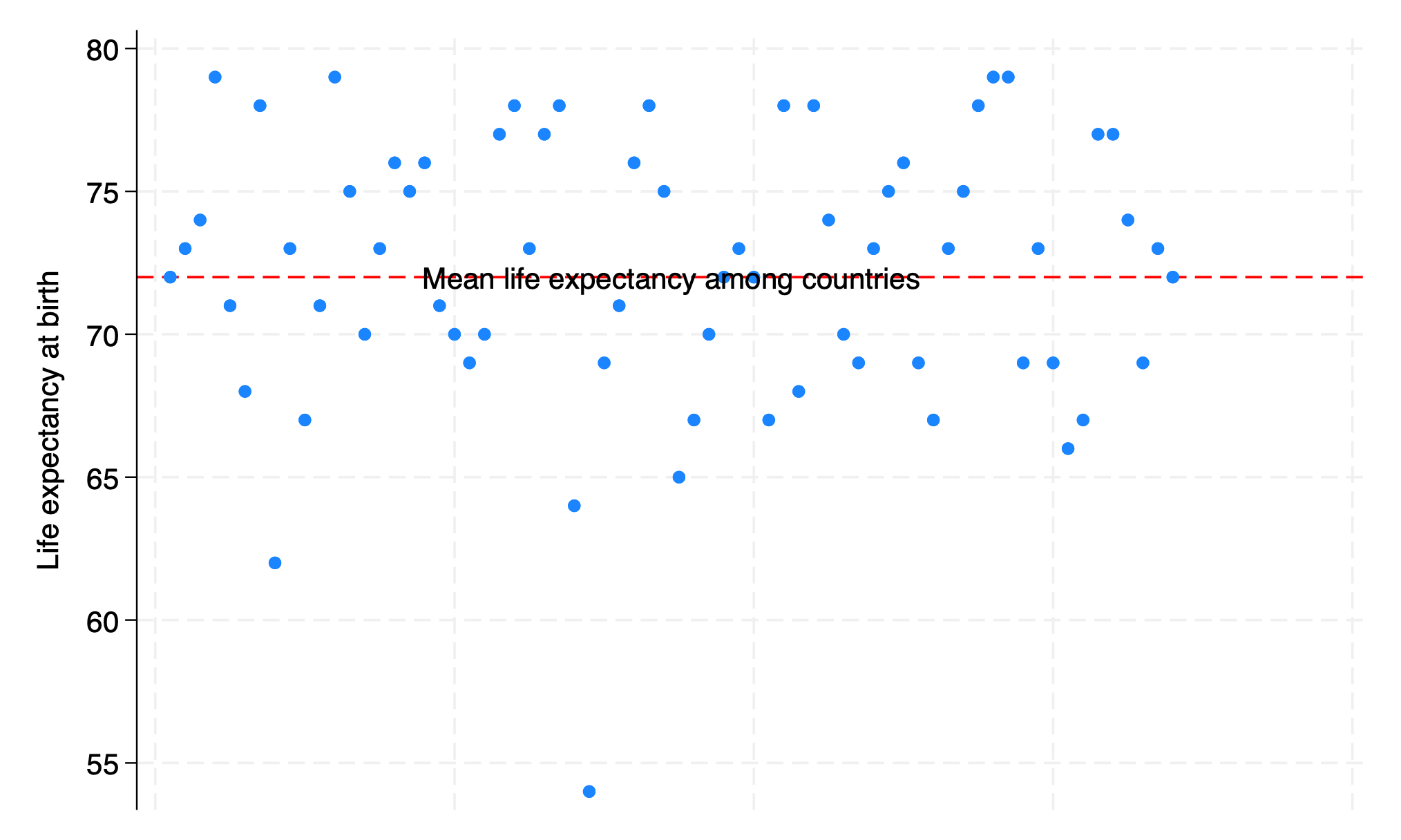
. twoway scatter lexp Country, ///
> xscale(off) ///
> yline(`lexp_mean', ///
> lc(red) ///
> lp(dash) ///
> ) ///
> text(`lexp_mean' `Country_mean' "Mean life expectancy among countries")
. graph export lexp_bycountry.png, replace
file /Users/d/Desktop/lexp_bycountry.png saved as PNG format
.
end of do-file
.
. qui {

.
. display c(N)
68

. display c(k)
6

. list in 1/5


    region	            country	    popgro~h	 lexp	    gnppc  safewa~r

1.  Europe & C. Asia	Albania	       1.2	        72	    810	    76
2.  Europe & C. Asia	Armenia	       1.1	        74	    460	    .
3.  Europe & C. Asia	Austria	       .4	        79	    26830   .
4.  Europe & C. Asia	Azerbaijan    1.4	        71	    480	    .
5.  Europe & C. Asia	Belarus	       .3	        68	    2180    .


.
end of do-file

.
Results: We identified the newly created .html file in our folder and opened it to compare its format to this markdown file. And we saw all that we had made, and behold, it was very good. Ghastly macros in the original markdown language now appeared as neatly formatted results. There were 68 observations and 6 observations in the analyzed dataset. Average life expectancy of all countries, \(\beta_0\), was 72 years. Difference in life expectancy among adjacent countries, \(\beta_1\), showed no trend or pattern and was 0.002 year, essentially \(zero\), and \(p = .95\)
Conclusions: In walking you through syntax, do-file creation, queued commands, generated results, through to embedding neatly formatted output in .html, we believe you now have a solid sense of all that Stata has to offer you. These ideas can be generalized to embedding results in .xlsx, .log, .dta, .docx, etc.
2.5 html#
2.5.1. How to embed Stata results in .html#
Author, MD MPH#
Background:
A user downloads and installs a system of program files, mostly ado-files, which form the foundation of most of the commands
used in Stata Programming. Using those commands and additional syntax written out sequentially in a do-file, the user creates
well-formed instruction to Stata called a do-file script. Once the user runs this script, results are generated and displayed
in the results window, in a graph, or in a format (.xlsx, .log, .dta, .docx, .md, LaTeX, .html, etc). The .html file format is of specific
interest since its the pathway to self-publication. To illustrate how this may be achieved in Stata, we hereby introduce the dyndoc
command.
Methods:
We created a do-file and populated it with this abstract using markdown language. Anything
in this document that is not ordinary text including <<dd_version: 2>>, <<dd_do:nooutput>>, <</dd_do>>, <<dd_display: c(N)>> is a
markup.
Results that might be numeric, string, alphanumeric, or formatted as macros are embeded at these markedup points. We then saved this
document using the file extension .do; however, any text file extension will work (.txt, .md, .do, etc). To the pwd where we saved
this text file, we added a cascading style sheet stmarkdown.css and header.txt to enhance the aesthetic of our .html file. Finally, we typed the
following command into the Stata command window: dyndoc filename.do, saving(filename.html) replace. In the key analysis, \(Y = \beta_0 + \beta_1 X\), where \(Y\) is life expectancy at birth in years, the outcome or dependent variable; \(X\) is the country, the predictor or independent variable being tested.
. webuse lifeexp, clear
(Life expectancy, 1998)

. encode country, gen(Country)

. quietly sum lexp

. qui local lexp_mean: di %3.0f r(mean)

. quietly sum Country

. qui local Country_mean: di r(mean)

. twoway scatter lexp Country, ///
>    xscale(off) ///
>    yline(`lexp_mean', ///
>       lc(red) ///
>       lp(dash) ///
>    ) ///
>    text(`lexp_mean' `Country_mean' "Mean life expectancy among countries")

. graph export lexp_bycountry.png, replace
file /Users/d/Desktop/lexp_bycountry.png saved as PNG format

.
end of do-file

.
. qui {

.
. display c(N)
68

. display c(k)
6

. list in 1/5


    region	            country	    popgro~h	 lexp	    gnppc  safewa~r

1.  Europe & C. Asia	Albania	       1.2	        72	    810	    76
2.  Europe & C. Asia	Armenia	       1.1	        74	    460	    .
3.  Europe & C. Asia	Austria	       .4	        79	    26830   .
4.  Europe & C. Asia	Azerbaijan    1.4	        71	    480	    .
5.  Europe & C. Asia	Belarus	       .3	        68	    2180    .


.
end of do-file

.
Results: We identified the newly created .html file in our folder and opened it to compare its format to this markdown file. And we saw all that we had made, and behold, it was very good. Ghastly macros in the original markdown language now appeared as neatly formatted results. There were 68 observations and 6 observations in the analyzed dataset. Average life expectancy of all countries, \(\beta_0\), was 72 years. Difference in life expectancy among adjacent countries, \(\beta_1\), showed no trend or pattern and was 0.002 year, essentially \(zero\), and \(p = .95\)
Conclusions: In walking you through syntax, do-file creation, queued commands, generated results, through to embedding neatly formatted output in .html, we believe you now have a solid sense of all that Stata has to offer you. These ideas can be generalized to embedding results in .xlsx, .log, .dta, .docx, etc.
2.6 Lab#
Below we’ll intersperse the Stata code you used for hw1 with explanatory notes in a concise manner suitable for intermediate learners.
clear
cls
Note: Clears the current dataset from memory and the Stata command window to start with a clean slate.
if c(N) {
    // Inspired by Polack et al., NEJM 2020
    // Let's reverse engineer and simulate data based on their results
}
Note: The comment introduces the purpose of the simulation, inspired by a study on the efficacy of a COVID-19 vaccine.
if c(os)=="Windows" {
    global workdir "`c(pwd)'\"
}
else {
    global workdir "`c(pwd)'/"
}
Note: Sets a global variable workdir to the current working directory, accommodating both Windows and Unix-based systems by adjusting the path’s slashes.
capture log close
log using ${workdir}simulation.log, replace //this code may need debugging for those with spaces in their filepaths
Note: Closes any open log and starts a new log file to record the session’s output, ensuring all commands and results are saved for review.
set seed 340600
set obs 37706
Note: Initializes the random number generator to ensure reproducibility and sets the number of observations (participants) in the dataset to 37,706, matching the study’s scale.
g bnt=rbinomial(1,.5);
Note: Generates a binary variable bnt to simulate random assignment to the vaccine or placebo group with equal probability.
lab define Bnt 0 "Placebo" 1 "BNT162b2";
label values bnt Bnt;
Note: Labels the bnt variable for clarity: 0 as “Placebo” and 1 as “BNT162b2” (the vaccine).
gen female=rbinomial(1, .494);
Note: Simulates gender distribution among participants, with approximately 49.4% being female.
tempvar dem;
gen `dem'=round(runiform(0,100),.1);
Note: Creates a temporary variable dem to assist in generating a race distribution among participants based on specified probabilities.
gen age=(rt(_N)*9.25)+52;
replace age=runiform(16,91) if !inrange(age,16,91);
Note: Generates participant ages using a transformation of the t-distribution and ensures all ages fall within the 16-91 range by replacing outliers with uniformly distributed ages within the range.
g days=rweibull(.7,17,0) if bnt==0;
g covid=rbinomial(1, 162/21728) if bnt==0;
replace days=rweibull(.4,.8,0) if bnt==1;
replace covid=rbinomial(1, 14/21772) if bnt=1;
Note: Simulates the days until potential COVID-19 infection and whether an infection occurred, with different parameters for the vaccine and placebo groups to reflect the vaccine’s efficacy.
stset days, fail(covid) ;
Note: Prepares the dataset for survival analysis, specifying days as the time variable and covid as the failure event indicator.
sts graph, by(bnt);
Note: Generates a Kaplan-Meier survival curve by treatment group to visualize the difference in COVID-19 incidence over time.
stcox bnt;
Note: Fits a Cox proportional hazards model to assess the vaccine’s effect on the hazard of contracting COVID-19.
lab var bnt_id "Participant Identifier";
Note: Labels the variables with descriptive names for clarity in the dataset’s context.
save BNT162b2, replace
Note: Saves the simulated dataset for future use or analysis.
2.7 Homework#
A few instructions (this is due 04/11/24, but we’ll accept late submissions for hw2):
Open a new .do file editor
Write syntax to create a .log file
Additional syntax to create a simulated dataset
Just use the syntax from hw1; i.e.,
do "github URL/hw1/yourname.do"
Confirm that you have a simulated dataset
e.g.
di c(N)
Create Table 1 to describe the study population you created in your simulation last week (watch video from session 2).
To install
table1_fena.adofor your current session, use this syntax:
do "https://raw.githubusercontent.com/jhustata/basic/main/table1_fena.ado"
After you’ve done this, you may run the following syntax:
table1_fena , var("female race ethnicity country bmi") by(bnt) title("Table 1. Patient and demographic characteristics") excel("Table1") catt(15) missingness
How may you find the .xlsx file with Table 1?
pwd
ls -l
You’re done! So remember to close your log file with the command
log closeSubmit only your .do file. We’ll run your script on our machines to see if it works. Think of us as your remoate collaborators in Australia with THE real data, as contrasted with your simulated data.
Common Mistakes Seen in HW2
<ul>
    <li>Use of <code>quietly</code> to control output</li>
    <li>Line continuation for <code>table1_fena</code> syntax</li>
    <li>Code commenting and annotation were sparse</li>
    <li>File path, work directory, and end-user ambiguity (try deleting your local file to see if the code still works)</li>
    <li>For HW5-7, submit a <code>.do</code> file to Dropbox as well as a URL of the <code>.do</code> file on GitHub</li>
</ul>
2.8 Extra notes#
These notes aim to guide you through the specific syntax and functionalities you’ll need to effectively utilize the provided .ado file (URL/table1_fena.ado). This file is designed for creating descriptive statistics tables (classically referred to as “Table 1” in medical research) in Stata, with support for handling variables by types, managing missing data, and exporting results to Excel. The syntax and features encapsulated within this .ado file cover several custom commands designed for data manipulation, variable type detection, and table generation.
Understanding the table1_fena Program#
Command Structure and Options
The
table1_fenaprogram is initiated withqui {to run quietly without displaying intermediate results.The
syntaxcommand specifies the expected input format, including optional and required arguments:Optional arguments are enclosed in square brackets
[ ].Required arguments are not enclosed and include options for specifying variables (
var), stratification (by), and other functionalities like title naming (title), Excel file naming (excel), category thresholds (catt), and handling missingness.
Variable type detection and user prompts are integral for ensuring correct data analysis and interpretation.
Variable Type Detection and Modification
Detects variable types automatically and allows manual adjustments via user input, addressing binary, categorical, and continuous variables.
Utilizes global macros (
bin,cat,con) for variable classification, which are crucial for the correct statistical analysis and table presentation.
Generation of Descriptive Statistics Tables
Facilitates table generation based on the specified criteria, including stratification (
byvariable), and the handling of binary, categorical, and continuous variables differently to reflect common practices in descriptive statistics reporting.Offers support for Excel export, making it easier to share and present results.
Using the var_type, missing_detect, and ind_translator Programs (this is VERY advanced and you may ignore it)#
var_typeProgram: Automates the classification of variables into binary, categorical, and continuous types, essential for accurate data representation and analysis.missing_detectProgram: Checks for and reports missing variables in the dataset, a crucial step for data cleaning and integrity checks before analysis.ind_translatorProgram: A utility program for translating Excel column and row indices into Excel references, facilitating dynamic Excel output generation.
Excel File Generation and Formatting with table1_creation#
Command Options and Flow Control: Demonstrates comprehensive options for table customization, including titles, variable inclusion, and Excel formatting.
Dynamic Content Generation: Includes advanced scripting for dynamic generation of table contents based on the dataset’s characteristics and user specifications.
Output Customization: Offers extensive customization options for the output, including Excel file naming, variable type adjustments, and the inclusion of missingness information.
Key Takeaways for Students#
Syntax Familiarization: Understand the command structure and syntax required to use the .ado file effectively. Pay attention to optional and required parameters and their significance.
Data Preparation: Recognize the importance of variable type detection and the ability to manually adjust these settings for accurate data analysis.
Output Generation: Learn how to generate descriptive statistics tables tailored to specific research needs, including handling different variable types and exporting to Excel for presentation.
Coding Best Practices: Note the use of local and global macros, conditional logic, and loops for efficient data manipulation and analysis in Stata.
You are encouraged to experiment with the commands within the context of different datasets, emphasizing the importance of accurate data classification (string, numeric, and if numeric: binary, categorical, and continous) and the practicality of generating descriptive statistics tables for their research projects.