
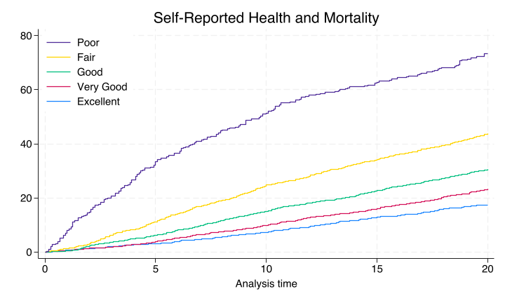
7. Survival analysis: non-parametric, semi-parametric, parametric#
7.1 Parameters#
Non-parametric#
Click to view the Stata code
cls
//1. data
global repo "https://github.com/jhustata/project/raw/main/"
global nhanes "https://wwwn.cdc.gov/Nchs/Nhanes/"

//2. code
do ${repo}followup.do
save followup, replace
import sasxport5 "${nhanes}1999-2000/DEMO.XPT", clear
merge 1:1 seqn using followup, nogen
save survey_followup, replace

//3. parameters
import sasxport5 "${nhanes}1999-2000/HUQ.XPT", clear
tab huq010
merge 1:1 seqn using survey_followup, nogen keep(matched)
rm followup.dta
rm survey_followup.dta
g years=permth_int/12
stset years, fail(mortstat)
replace huq010=. if huq010==9
label define huq 1 "Excellent" 2 "Very Good" 3 "Good" 4 "Fair" 5 "Poor"
label values huq010 huq
levelsof huq010, local(numlevels)
local i=1
foreach l of numlist `numlevels' {
    local vallab: value label huq010
	local catlab: lab `vallab' `l'
	global legend`i' = "`catlab'"
	local i= `i' + 1
}
save week7, replace
sts graph, ///
    by(huq010) ///
	fail ///
	per(100) ///
	ylab(0(20)80 , ///
	    format(%2.0f) ///
	) ///
	xlab(0(5)20) ///
	tmax(20) ///
	ti("Self-Reported Health and Mortality") ///
	legend( ///
	    order(5 4 3 2 1) ///
		lab(1 "$legend1") ///
		lab(2 "$legend2") ///
		lab(3 "$legend3") ///
		lab(4 "$legend4") ///
		lab(5 "$legend5") ///
		ring(0) pos(11) ///
	)
graph export nonpara.png, replace
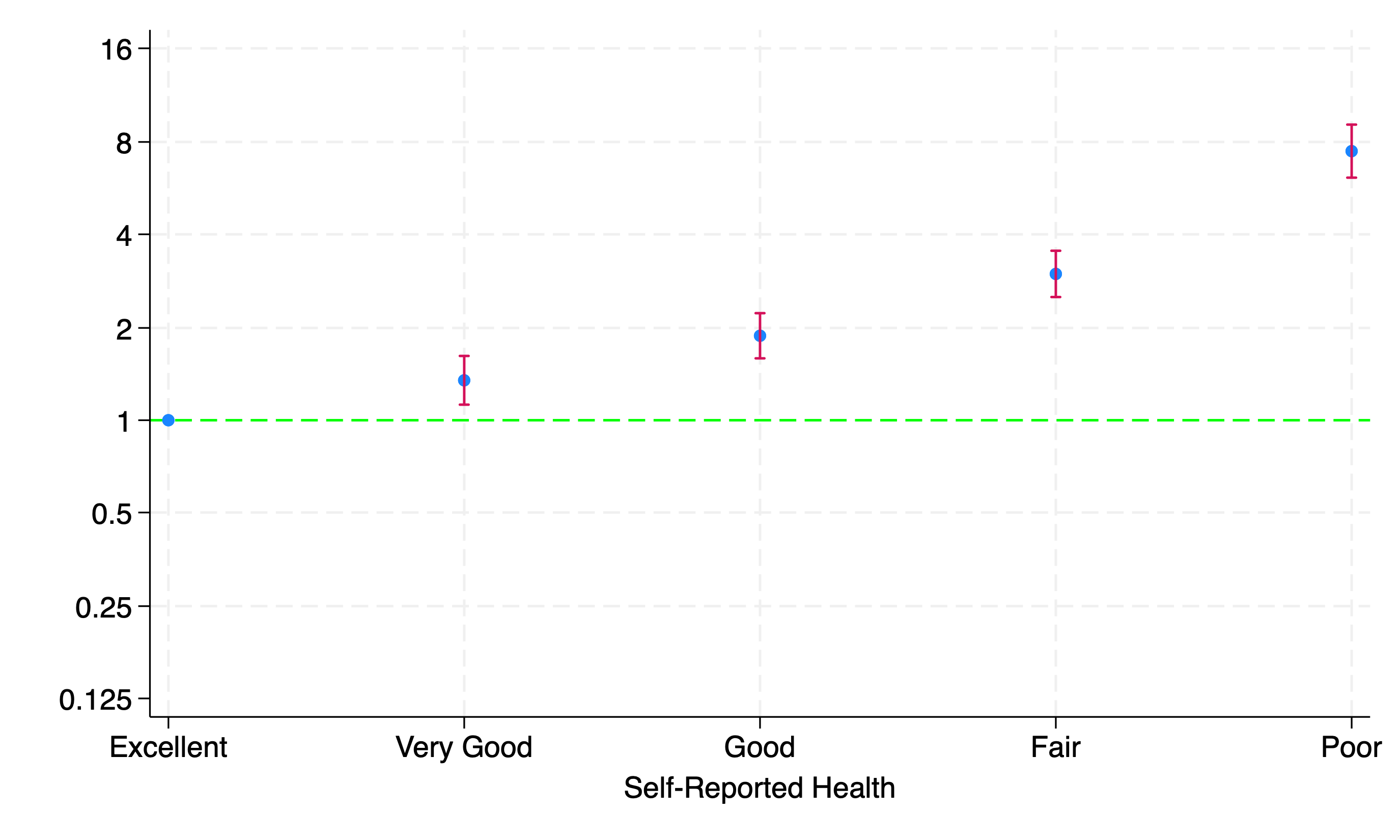
Semi-parametric#
Click to view the Stata code
/* -- earlier code --*/
stcox i.huq010, basesurv(s0)
matrix define mat = r(table)
matrix list mat
matrix mat = mat'
svmat mat
preserve
keep mat*
drop if missing(mat1)
rename (mat1 mat2 mat3 mat4 mat5 mat6 mat7 mat8 mat9)(b se z p ll ul df crit eform)
g x=_n
replace b=log(b)
replace ll=log(ll)
replace ul=log(ul)
twoway (scatter b x) || ///
       (rcap ll ul x, ///
	       yline(0, lcol(lime)) ///
		   ylab( ///
		       -2.08 "0.125" ///
			   -1.39 "0.25" ///
			   -.69 "0.5" ///
			     0 "1"  ///
			   .69 "2" ///
			   1.39 "4" ///
			   2.08 "8" ///
			   2.78 "16") ///
		   legend(off)  ///
		xlab( ///
           1 "$legend1" ///
		   2 "$legend2" ///
		   3 "$legend3" ///
		   4 "$legend4" ///
		   5 "$legend5") ///
	   xti("Self-Reported Health") ///
	   	   )
graph export semipara_unadj.png, replace
graph save semipara_unadj.gph, replace
restore
7.2 Inferences#
Click to view the Stata code
hist ridageyr
graph export nonpara.png, replace
//replace ridageyr=ridageyr/10
capture drop s0
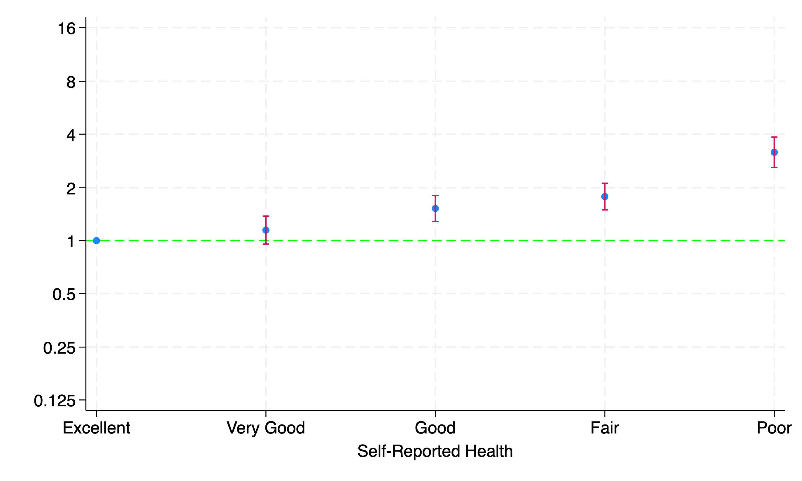
stcox i.huq010 ridageyr riagendr, basesurv(s0)
return list
matrix define mat_adj=r(table)
matrix define mat_adj=mat_adj'
matrix list mat_adj
svmat mat_adj
keep mat_adj*
drop if missing(mat_adj1)
rename (mat_adj1 mat_adj2 mat_adj3 mat_adj4 mat_adj5 mat_adj6 mat_adj7 mat_adj8 mat_adj9)(b se z p ll ul df crit eform)
g x=_n
replace b=log(b)
replace ll=log(ll)
replace ul=log(ul)
twoway (scatter b x if inrange(x,1,5)) || ///
(rcap ll ul x if inrange(x,1,5), ///
yline(0, lcol(lime)) ///
ylab( ///
-2.08 "0.125" ///
-1.39 "0.25" ///
-.69 "0.5" ///
0 "1" ///
.69 "2" ///
1.39 "4" ///
2.08 "8" ///
2.78 "16") ///
legend(off) ///
xlab( ///
1 "$legend1" ///
2 "$legend2" ///
3 "$legend3" ///
4 "$legend4" ///
5 "$legend5") ///
xti("Self-Reported Health") ///
)
graph export semipara_adj.png, replace
graph save semipara_adj.gph, replace
\(H_a: \text{Self-reported health} \sim Age\)#
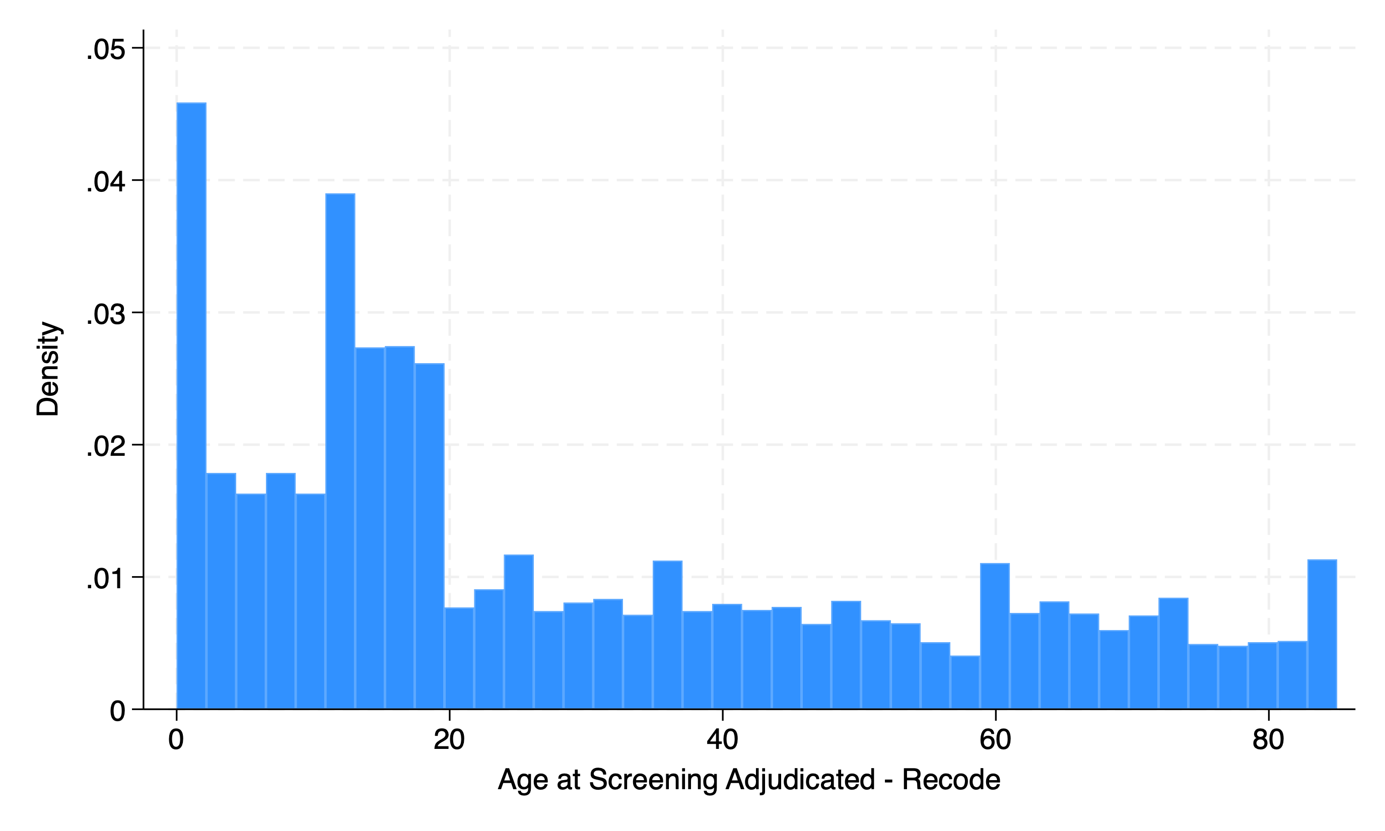
Adjust for age and other demographics#
7.3 Updates#
Comment on the coefficients of the parameters in the unadjusted analysis
What is the impact on your inferences of accounting for age, sex and race?
Are you content with your inferences after adjusting for demographics?
Might there be other potential confounders from questionnaire, exam, and labs?
How might you prepare the updated analysis to take additional variables into consideration?
You might already know that you lose degrees of freedom as you add parameters to your model
So how about increasing your “freedoms” by having a larger population size? Could you write a script that allows any “visitor” to your website or repo to test this hypothesis on a larger study population, taking into account additional survey years?
This latter issue is the definitive update for week 8 of the class
graph combine semipara_unadj.gph semipara_adj.gph, ///
    ycommon ti("Hazard Ratio, 95%CI")
graph export unadj_adj.png, replace

//these variable names don't exist in the dataset, this is a mere demo
di "What do you wish to adjust for in this analysis?" _request($varlist)
capture program drop selfassess
program define selfassess
    syntax varlist
    stcox i.huq010 `varlist'
end
selfassess $varlist
In the above example, you might ask your collaborators to list what they believe might be confounders in the assocation between self-assessed health status and mortality
7.4 Transparency#
The “most open” you can ever get in the “Open Science” enterprise is by using a public GitHub repo
Of the topics we’ve discussed, including data, code, parameters, inferences, and updates, “data” is of particular concern if there might be “disclosure risks”
In the Stata II (Intermediate) we’ll assume all data are de-identified and have zero disclosure risk. Perhaps because we’ve de-identified the data or because we are using simulated datasets
But in Stata III (Advanced) we’ll learn how to use private repos for data storage. We’ll consider how to grant limited access by means of temporary “tokens”
Regardless, the parameters of our models represent reduced dimensions of data and have no associated disclosure risks
So we should consider “extracting” parameters from our data and from that point forth being 100% transparent in our workflow
7.5 Extracting Parameters#
Virtually all scientific inferences from quantitive analyses can be made as long as you have the beta coefficients and the variance-covariance matrix following a multivariable regression.
Because these parameters have zero discolure risk, you are encouraged to have them made available to the public in your public GitHub repo
You’d do the public an extra favor if you laid out a generalizable program that allows anyone to add new parameters (i.e., variables and interactions amongst them) to the model with little extra effort
Let’s restore the analytic dataset we’d created. If this dataset has disclosure risks, the we should extract “all” the relevant parameters for statistical inference, make them publically available, and display our findings
cls
use week7, clear
e(b)#
Click to view the Stata code
cls
use week7, clear
replace riagendr=riagendr-1
stcox i.huq010 ridageyr riagendr, basesurv(s0)
keep s0 _t _t0 _st _d
save s0, replace
ereturn list
matrix beta = e(b)
matrix vcov = e(V)
matrix SV = ( ///
0, ///
1, ///
0, ///
0, ///
0, ///
40, ///
1 ///
)
matrix SV_ref = ( ///
0, ///
1, ///
0, ///
0, ///
0, ///
60, ///
1 ///
)
//absolute risk
matrix risk_score = SV * beta'
matrix list risk_score
di exp(risk_score[1,1])
matrix var_prediction = SV * vcov * vcov'
matrix se_prediction = sqrt(var_prediction[1,1])
matrix risk_score_ref = SV_ref * beta'
matrix list risk_score_ref
di exp(risk_score_ref[1,1])
matrix var_prediction_ref = SV_ref * vcov * vcov'
matrix se_prediction_ref = sqrt(var_prediction_ref[1,1])
local hr = exp(risk_score_ref[1,1])/exp(risk_score[1,1])
di `hr'
//di "We conclude that `exp(risk_score[1,1])'"
//
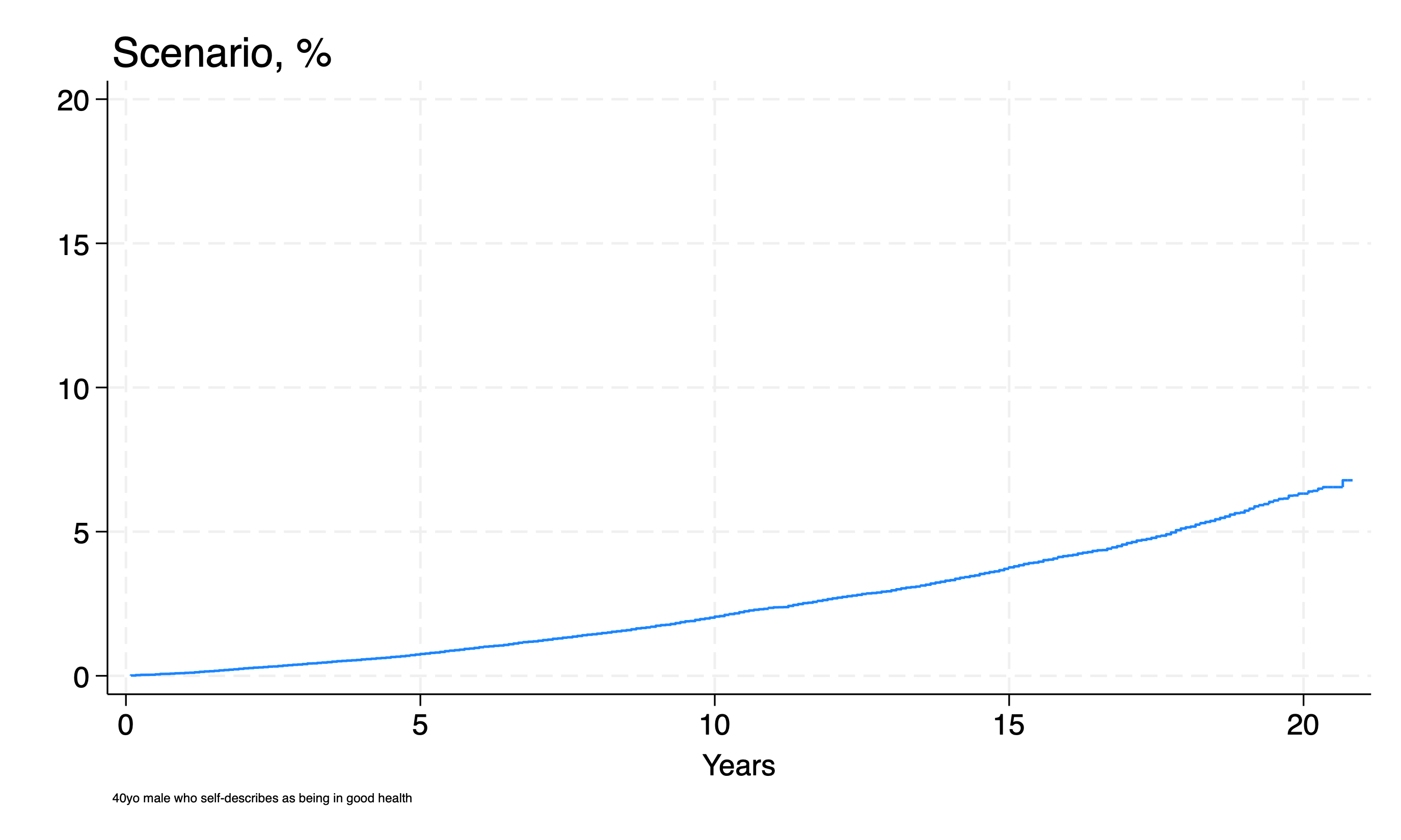
g f0 = (1 - s0) * 100
g f1_ = f0 * exp(risk_score[1,1])
line f1 _t , ///
sort connect(step step) ///
legend(ring(0)) ///
ylab(0(5)20) xlab(0(5)20) ///
yti("") ///
ti("Scenario, %", pos(11)) ///
xti("Years") ///
note("40yo male who self-describes as being in good health" ///
,size(1.5) ///
)
graph export scenario.png, replace
e(V)#
Estimating the 95%CI interval for specific scenarios is beyond the scope of this class and will be left to Stata III (Advanced)
7.6 Lab#
Objective: Prepare and analyze the data from last week’s lab (Lab 6) using nonparametric (Kaplan-Meier), semiparametric (Cox Regression), and parametric (Weibull regression) methods. Generate figures to illustrate absolute risks (cumulative incidence) and relative risks (hazard ratios). Consider adjusting for age, sex, race, and two additional confounders to achieve unbiased inferences. Merge your analytic dataset with additional datasets containing these variables, which you can find on the NHANES website. Consider how your experience with NHANES can inform improvements to your website.
Examples of datasets you may merge with the master analytic dataset include:
// Questionnaire data: includes "Doctor told you have diabetes"
import sasxport5 "${nhanes}1999-2000//DIQ.XPT", clear

// Exam data: includes systolic and diastolic blood pressure
import sasxport5 "${nhanes}1999-2000/BPX.XPT"

// Lab data: includes serum creatinine
import sasxport5 "${nhanes}1999-2000/LAB16.XPT", clear
Provide documentation on your homepage and include necessary links to help visitors navigate your website efficiently.
7.7 Homework#
Generate .html files of your Stata output using the dyndoc command and provide links to this Stata output on your website to showcase the richness of your output.
You can also document your Stata code without using dyndoc by creating other .md files with annotations and notes interspersed with Stata code, similar to how this classbook is structured.
For this Stata Programming II (Intermediate) class, however, you must create a separate website with output directly from Stata. Include a link to this dyndoc output on your homepage.
To do this:
Upload output from running nonparametric and semiparametric estimates in Stata using the
dyndoccommand. Save the created file and additional output asdyndoc.html, then upload it to your project repo.Use markdown syntax within
index.mdto help visitors navigate to this output. You can use syntax like the example below:
click [here](dyndoc.html) to view nonparametric and semiparametric risk estimates from Stata
Keep your homepage (
index.md) tidy and informative without being cluttered. Use hyperlinks like the one above to invite readers to explore specific aspects of your data, code, parameters, inferences, updates, or any other aspect of your project that enhances transparency and reproducibility.