
8. Finesse project website, reduce clutter, ensure reproducibility#
8.1 Finesse project website#
A project website might be a reflection of your professionalism and attention to detail. Ensure that your website is easy to navigate, with clear menus and a cohesive design.
8.2 Reduce clutter#
Clarity is key in clinical and public health research communications. Use hyperlinks to provide detailed information on a separate webpage, keeping your main page clean and focused. This allows readers to explore topics in more depth if they wish.
8.3 Ensure reprodicibility#
Reproducibility is the cornerstone of scientific research. Document your code and data sources meticulously, and provide clear instructions for running analyses. This allows others to replicate your findings.
Show code cell source
//cls
qui {
	if 1 {
//1. data
global repo "https://github.com/jhustata/project/raw/main/"
global nhanes "https://wwwn.cdc.gov/Nchs/Nhanes/"

//2. code
do ${repo}followup.do
save ~/documents/github/statatwo/followup, replace
import sasxport5 "${nhanes}1999-2000/DEMO.XPT", clear
merge 1:1 seqn using followup, nogen
save ~/documents/github/statatwo/survey_followup, replace

//3. parameters
import sasxport5 "${nhanes}1999-2000/HUQ.XPT", clear
tab huq010
merge 1:1 seqn using ~/documents/github/statatwo/survey_followup, nogen keep(matched)
rm ~/documents/github/statatwo/followup.dta
rm ~/documents/github/statatwo/survey_followup.dta
g years=permth_int/12
stset years, fail(mortstat)
replace huq010=. if huq010==9
label define huq 1 "Excellent" 2 "Very Good" 3 "Good" 4 "Fair" 5 "Poor"
label values huq010 huq
levelsof huq010, local(numlevels)
local i=1
foreach l of numlist `numlevels' {
    local vallab: value label huq010
	local catlab: lab `vallab' `l'
	global legend`i' = "`catlab'"
	local i= `i' + 1
}
save ~/documents/github/statatwo/week7, replace
#delimit;
sts graph,
    by(huq010)
	fail
	per(100)
	ylab(0(20)80 ,
	    format(%2.0f)
	)
	xlab(0(5)20)
	tmax(20)
	ti("Self-Reported Health and Mortality")
	legend(
	    order(5 4 3 2 1)
		lab(1 "$legend1")
		lab(2 "$legend2")
		lab(3 "$legend3")
		lab(4 "$legend4")
		lab(5 "$legend5")
		ring(0) pos(11)
	) ;
#delimit cr
graph export ~/documents/github/statatwo/nonpara.png, replace
save ~/documents/github/statatwo/wk8, replace
    }
}
use ~/documents/github/statatwo/wk8, clear
stcox i.huq010, basesurv(s0)
sort _t s0
list _t s0 in 1/20
keep _t s0
save ~/documents/github/statatwo/s0, replace
Show code cell output
file /Users/apollo/documents/github/statatwo/followup.dta could not be opened
r(603);
r(603);
foreach n of numlist 1 1.34 1.88 2.98 7.47 {
	di log(`n')
}
0
.29266961
.63127178
1.0919233
2.010895
Show code cell source
list if inrange(_t, 0, .000001)
list if inrange(_t, 4.999999, 5.000001)
list if inrange(_t, 9.999999, 10.000001)
list if inrange(_t, 14.999999, 15.000001)
list if inrange(_t, 19.999999, 20.000001)
Show code cell output
      +----------------+
      | _t          s0 |
      |----------------|
 394. |  5   .96281503 |
 395. |  5   .96281503 |
 396. |  5   .96281503 |
 397. |  5   .96281503 |
 398. |  5   .96281503 |
      |----------------|
 399. |  5   .96281503 |
 400. |  5   .96281503 |
 401. |  5   .96281503 |
 402. |  5   .96281503 |
      +----------------+


      +----------------+
      | _t          s0 |
      |----------------|
 863. | 10   .91558171 |
 864. | 10   .91558171 |
 865. | 10   .91558171 |
 866. | 10   .91558171 |
 867. | 10   .91558171 |
      |----------------|
 868. | 10   .91558171 |
 869. | 10   .91558171 |
 870. | 10   .91558171 |
      +----------------+


      +----------------+
      | _t          s0 |
      |----------------|
1264. | 15   .87179276 |
1265. | 15   .87179276 |
1266. | 15   .87179276 |
1267. | 15   .87179276 |
1268. | 15   .87179276 |
      |----------------|
1269. | 15   .87179276 |
1270. | 15   .87179276 |
1271. | 15   .87179276 |
1272. | 15   .87179276 |
      +----------------+


      +----------------+
      | _t          s0 |
      |----------------|
3557. | 20   .82403985 |
3558. | 20   .82403985 |
3559. | 20   .82403985 |
3560. | 20   .82403985 |
3561. | 20   .82403985 |
      |----------------|
3562. | 20   .82403985 |
3563. | 20   .82403985 |
3564. | 20   .82403985 |
3565. | 20   .82403985 |
3566. | 20   .82403985 |
      |----------------|
3567. | 20   .82403985 |
3568. | 20   .82403985 |
3569. | 20   .82403985 |
3570. | 20   .82403985 |
3571. | 20   .82403985 |
      |----------------|
3572. | 20   .82403985 |
3573. | 20   .82403985 |
3574. | 20   .82403985 |
3575. | 20   .82403985 |
3576. | 20   .82403985 |
      |----------------|
3577. | 20   .82403985 |
3578. | 20   .82403985 |
3579. | 20   .82403985 |
3580. | 20   .82403985 |
3581. | 20   .82403985 |
      |----------------|
3582. | 20   .82403985 |
3583. | 20   .82403985 |
3584. | 20   .82403985 |
3585. | 20   .82403985 |
3586. | 20   .82403985 |
      |----------------|
3587. | 20   .82403985 |
3588. | 20   .82403985 |
3589. | 20   .82403985 |
3590. | 20   .82403985 |
3591. | 20   .82403985 |
      |----------------|
3592. | 20   .82403985 |
3593. | 20   .82403985 |
3594. | 20   .82403985 |
3595. | 20   .82403985 |
3596. | 20   .82403985 |
      |----------------|
3597. | 20   .82403985 |
3598. | 20   .82403985 |
3599. | 20   .82403985 |
3600. | 20   .82403985 |
3601. | 20   .82403985 |
      |----------------|
3602. | 20   .82403985 |
3603. | 20   .82403985 |
3604. | 20   .82403985 |
3605. | 20   .82403985 |
3606. | 20   .82403985 |
      |----------------|
3607. | 20   .82403985 |
3608. | 20   .82403985 |
3609. | 20   .82403985 |
3610. | 20   .82403985 |
3611. | 20   .82403985 |
      |----------------|
3612. | 20   .82403985 |
3613. | 20   .82403985 |
3614. | 20   .82403985 |
3615. | 20   .82403985 |
3616. | 20   .82403985 |
      |----------------|
3617. | 20   .82403985 |
3618. | 20   .82403985 |
3619. | 20   .82403985 |
3620. | 20   .82403985 |
3621. | 20   .82403985 |
      |----------------|
3622. | 20   .82403985 |
3623. | 20   .82403985 |
3624. | 20   .82403985 |
3625. | 20   .82403985 |
3626. | 20   .82403985 |
      |----------------|
3627. | 20   .82403985 |
3628. | 20   .82403985 |
3629. | 20   .82403985 |
3630. | 20   .82403985 |
3631. | 20   .82403985 |
      |----------------|
3632. | 20   .82403985 |
3633. | 20   .82403985 |
3634. | 20   .82403985 |
3635. | 20   .82403985 |
3636. | 20   .82403985 |
      |----------------|
--more--
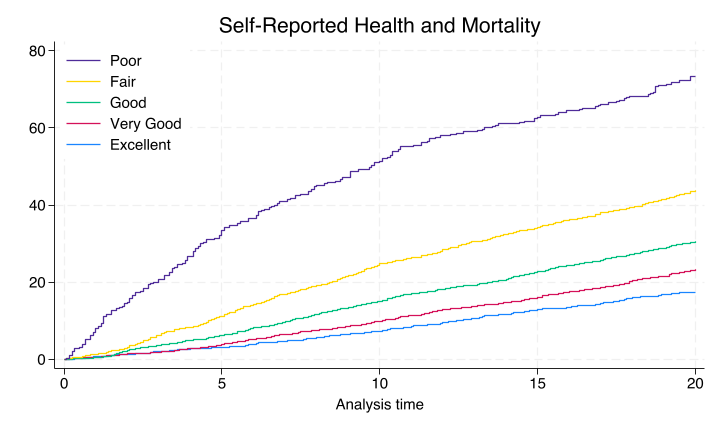
Nonparametric#
This line of code graph export ~/documents/github/statatwo/nonpara.png, replace above yields the nonparametric product-limit-estimator, also known as the “Kaplan-Meier” curve seen below.
Semiparametric#
The results from a Cox regression above, stcox i.huq010, basesurv(s0), are semi-parametric. The \(\beta_i\) coefficients for the hug010 categories are the parametric moiety, where as the \(s0\) kaplan-meier estimate for the basecase is the nonparametic; hence, semiparametric!
qui {
matrix b = e(b)
matrix list b
//SV -> scenario vector (i.e., user-input = scenario)
//In the scenario below b0=1, b1=0, b2=0, b3=0, b4=0m b5=0
matrix define SV = (1, 0, 0, 0, 0)
//yields the logHR
matrix loghr = SV*b'
use "${repo}s0.dta", clear
g f0 = (1 - s0)*100
g f1 = f0*exp(loghr[1,1])
noi sum f1 if inrange(_t,0,.0001)
noi sum f1 if inrange(_t,4.9999,5.0001)
noi sum f1 if inrange(_t,9.9999,10.0001)
noi sum f1 if inrange(_t,14.9999,15.0001)
noi sum f1 if inrange(_t,19.9999,20.0001)
//Segev, JAMA, 2010
noi di "Donor mortality at 12-year follow-up:" %3.1f r(max) "%"
#delimit;
line f1 _t if inrange(_t,1,15),
    sort
	connect(step step)
	ylab(0(10)40,
	    format(%2.0f)
	)
	xlab(0(3)15)
	yti("%")
	xti("Years")
	;
#delimit cr
}