2. Return values, macros, programs

2.0 Last week

Let’s briefly recap what we covered last week (survey, overview) and what you’ve practiced this week in lab:

1. Importing data

2. Performing basic queries

3. Outputing some of your findings into .xlsx, .log, etc.

   • We’ll do more of this later

Today we’ll build on these ideas:

1. String values as output

   • survey

2. Numeric values embedded within a string

   • Using macros

     • System

       • creturn list

       • return list

       • ereturn list

     • User-defined

       • Global

         • global workdir c(pwd)

       • Local

         • local mean: di %3.1f r(mean)

3. Examples beyond .xlsx and .dta

4. Programs

   program define myfirstprogram
      di "Hello, Class!"
   end

Show code cell source Hide code cell source

import networkx as nx
import matplotlib.pyplot as plt
#import numpy as np
#import sklearn as skl
# 

#plt.figure(figsize=[2, 2])
G = nx.DiGraph()
G.add_node("user",  pos = (550,500) )
G.add_node("system",  pos = (-550,500) )
G.add_node("program",  pos = (-2000, 960) )
G.add_node("syntax",  pos = (2000, 950) )
G.add_node("ado", pos = (-3000, 550) )
G.add_node("do", pos = (3000, 550) )
G.add_node("command", pos = (-1900, 150) )
G.add_node("queue", pos = (1900, 150) )
G.add_node("results", pos = (0,0))
G.add_node("dta", pos = (0, -475))
G.add_node("log", pos = (-1900, -475))
G.add_node("excel", pos = (-4000, -475))
G.add_node("word", pos = (1900, -475))
G.add_node("html", pos = (4000, -475))
G.add_node("publish", pos = (0, -950))
G.add_edges_from([ ("program","ado"), ("syntax", "do")])
G.add_edges_from([("ado", "command"), ("do", "queue") ])
G.add_edges_from([("command", "results"), ("queue", "results"),("results","excel"),("results","word"),("results","html")])
G.add_edges_from([("results","dta"),("results","log")])
G.add_edges_from([("dta","publish"),("log","publish"),("excel","publish"),("word","publish"),("html","publish")])
nx.draw(G, 
        nx.get_node_attributes(G, 'pos'), 
        with_labels=True, 
        font_weight='bold', 
        node_size = 4500,
        node_color = "lightblue",
        linewidths = 3)
ax= plt.gca()
ax.collections[0].set_edgecolor("#000000")
ax.set_xlim([-5000, 5000])
ax.set_ylim([-1000, 1000])
plt.show()

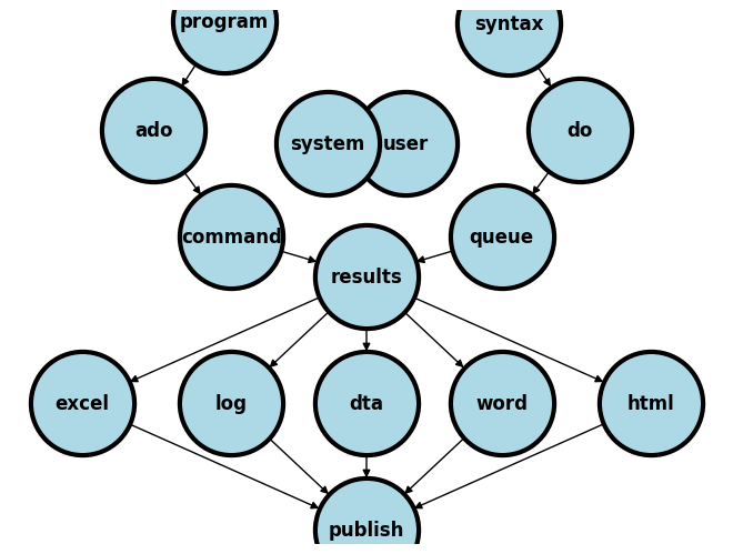
2.01 Results/output

• A sequence or queue of instructions commands + syntax = code given to Stata via a do-file will generate results

• Never include results in your do-file when you share your work in this class and with future collaborators

• Due diligence in the open-science enterprise demands that others reproduce your results and findings

• Your duty is to share only the input, and ours is to reproduce your output so as to fullfil our shared Credo

• Please share your do-files and any third-party ado-files, if at all your script or do-file relies on third-party programs

2.02 Display/files

• Stata’s Results Window

  • Only useful to the user

  • Not a mode of publication

• .xlsx

• .log

• .dta

• .docx

• .html

2.03 Examples

2.031 xlsx

Import a datafile

use transplants, clear 

Use the putexcel command to create an Excel spreadsheet and name it “table1.xlsx”

putexcel set table1, replace

Populate the first row and first column with the text “Table 1. Demographic and clinical characteristics of kidney transplant recipients”

putexcel A1="Table 1. Demographic and clinical characteristics of kidney transplant recipients"

Now populate the second row and first column with the total number of observations in the transplants.dta dataset

putexcel B1="N=`c(N)'"

Please engage with our new Stata-focused community, share what you know about the putexcel command, ask questions about this command, and contribute solutions to posted problems.

Copy and paste the code snippet under the title “Sharing Code” into your .do file and run the script. Are you able to find your output?

If you get an error, it’s likely that you did not edit the file path in the code. Always remember to adapt borrrowed code to your needs!

2.032 log

Let’s input some Stata code into your .do file. The transplants.dta datafile is here for your convenience. You may download it to use it locally or use the URL to import the data directly from the remote location.

capture log close
log using chi2.log, replace //creates a .log file
use transplants, clear //imports the datafile
tab dx gender, row  chi2 //performs a chi-square test
log close //closes the .log file

Now lets find the content of the .log file created. When analyzing data in Stata, one often encounters the need to review or share results in a format that is both informative and easily interpretable. An essential step in this process involves examining the output stored in log-files. These files capture the essence of your analytical work, including statistical tests and their results. A common feature of interest in these results is the p-value, a metric that helps us understand the significance of our findings.

. tab dx gender, row  chi2

+----------------+
Key            
------------------
frequency    
row percentage 
+----------------+

Primary            gender
Diagnosis      |    0    |    1	    | Total
---------------+---------+----------+------			
1=Glomerular   |  237    |    187   |	 424 
               |  55.90  |   44.10  | 100.00 
---------------+---------+----------+------			
2=Diabetes     | 60      |  37	    | 97 
               | 61.86   |  38.14   | 100.00 
---------------+---------+----------+------			
3=PKD          | 81      |  66	    | 147 
               | 55.10   |  44.90   | 100.00 
---------------+---------+----------+------			
4=Hypertensive | 316     |  176	    | 492 
               | 64.23   |  35.77   | 100.00 
---------------+---------+----------+------		
5=Renovascular | 24      |  15	    | 39 
               | 61.54   |  38.46   | 100.00 
---------------+---------+----------+------			
6=Congenital   | 46      |  22	    | 68 
               | 67.65   |  32.35   | 100.00 
---------------+---------+----------+------				
7=Tubulo       | 32      |  35	    | 67 
               | 47.76   |  52.24   | 100.00 
---------------+---------+----------+------			
8=Neoplasm     | 8       |  5	    | 13 
               | 61.54   |  38.46   | 100.00 
---------------+---------+----------+------			
9=Other        | 421     |  232	    | 653 
               | 64.47   |  35.53   | 100.00 
---------------+---------+----------+------			
Total          | 1,225   |  775     | 2,000 
               | 61.25   |  38.75   | 100.00 

Pearson chi2(8) =  18.4805	Pr	= 0.018

. 

To start, let’s consider the return list command:

return list

This command is your gateway to reviewing the most recent test results stored by Stata. It lists out all the statistics calculated by the last command, including the number of observations (r(N)), test statistics like chi-squared values (r(chi2)), and crucially, the p-value (r(p)).

However, simply listing out the p-value isn’t always enough, especially when preparing your findings for a broader audience, such as in peer-reviewed publications. The reporting of p-values follows specific conventions to enhance clarity and understanding. Let’s explore how to apply these conventions using a conditional formatting approach:

Introduction to the “quietly” Command

The first block introduces the concept of running commands ‘quietly’ in Stata, which suppresses the output in the Results window.

qui {
    // Your Stata commands here
} 

• qui {: This command is short for ‘quietly’. It tells Stata to execute the commands within the braces without displaying the usual output in the Results window. It’s helpful for keeping your results clean or when you’re only interested in the final outcome rather than seeing every step.

• }: This closing brace marks the end of the ‘quietly’ section. After this point, Stata will return to its default behavior, which is to display output for each command.

Handling p-values Less Than 0.01

The second block explains how to handle cases where p-values are less than 0.01.

qui {
    if r(p) < 0.01 {
        local p: di "p < 0.01"
    }
}

• if r(p) < 0.01 {: This line checks if the p-value (r(p)) from the last statistical test is less than 0.01. If true, the commands inside the braces will execute.

• local p: di "p < 0.01": Here, if the condition is met, we assign a formatted string “p < 0.01” to a local macro named p. This is a concise way to communicate that the test results are highly significant.

Formatting p-values Between 0.01 and 0.05

The third block focuses on p-values that fall between 0.01 and 0.05, using precision formatting.

qui {
    else if inrange(r(p),0.01,0.05) {
        local p: di %3.2f r(p)
    }
}

• else if inrange(r(p),0.01,0.05) {: This line checks if the p-value is within the specified range. The inrange() function is versatile, allowing for clear boundary definitions.

• local p: di %3.2f r(p): For p-values in this range, we format the number to have two decimal places (e.g., 0.03), ensuring clarity and precision in our reporting.

Formatting p-values Greater Than 0.05

The fourth block deals with formatting p-values greater than 0.05.

qui {
    else {
        local p: di %2.1f r(p)
    }
}

• else {: This part catches any cases not previously covered, essentially p-values greater than 0.05.

• local p: di %2.1f r(p): Here, we format the p-value to have one decimal place, indicating a less strict interpretation of statistical significance.

Combining Everything

Finally, we combine all the parts into a cohesive whole, demonstrating how to format p-values based on their value, all within a ‘quietly’ block.

qui { //asks Stata to work "quietly", until the corresponding brace is closed at the end

    capture log close
    log using chi2.log, replace //creates a .log file
    use transplants, clear //imports the datafile
    tab dx gender, row  chi2 //performs a chi-square test

    if r(p) < 0.01 {
       local p: di "p < 0.01"
    }
    else if inrange(r(p),0.01,0.05) {
       local p: di %3.2f r(p)
    }
    else {
       local p: di %2.1f r(p)
    }
    noi di "p = `p'"
	log close //closes the .log file
} //after this brace Stata may return to its default: "noisely" produce output as it runs the program

• This final block puts everything together, showing how to use qui to suppress unnecessary output while precisely formatting p-values according to their significance level. The following line then displays the formatted p-value, completing the explanation of how to communicate statistical results clearly and effectively:

noi di "p = `p'"

Recap of the chi-square test

In this script, we start by checking if the p-value is less than 0.01. If so, we report it as “p < 0.01” to indicate a very high level of statistical significance. This convention signals to the reader that the result is significant beyond the conventional thresholds.

If the p-value falls between 0.01 and 0.05, we report it in a standard numeric format (e.g., 0.03), maintaining two decimal places for precision. This range indicates statistical significance at the conventional 5% level, which is widely accepted in many research disciplines.

For p-values greater than 0.05, we format them with one decimal place, acknowledging that while the result may not meet the conventional threshold for statistical significance, it is still worth reporting for a comprehensive understanding of the analysis.

This approach to formatting and reporting p-values is not just about following academic conventions; it’s about making your results clear and interpretable for your audience, facilitating better understanding and discussion of your research findings.

In practice, here’s how the output might look after applying our formatting script:

. return list 

scalars:
r(N) =  2000
r(r) =  9
r(c) =  2
r(chi2) =  18.48047641017726
r(p) =  .0178990677414798

. qui {
p = 0.02

Notice how the p-value is processed and reported as “0.02” to fit the specified format for p-values between 0.01 and 0.05. This precision in reporting underscores the importance of statistical details in the broader narrative of your research findings.

chi2.log

2.033 dta

Step 1: Clearing the Workspace

cls
clear 
postutil clear 

• cls: Clears the Stata command window, providing a clean slate for your next commands. It’s a good practice to start with this to avoid confusion from previous outputs.

• clear: Removes all data from memory. This ensures that the workspace is clean before starting new data manipulations.

• postutil clear: Clears any existing posted datasets from memory. This is particularly useful when you’re about to create new posted datasets, ensuring no conflicts or errors arise from previous sessions.

Step 2: Setting Up a New Posted File

postfile pp str80 a float(b c) using output.dta, replace 

• postfile pp str80 a float(b c) using output.dta, replace: This line initiates the creation of a new dataset (output.dta) with specific variables a, b, and c. Here, pp is the name given to this posting session, str80 a defines a as a string variable with a maximum length of 80 characters, and float(b c) defines b and c as floating-point numbers. The replace option allows overwriting any existing file with the same name, ensuring that your new data is saved without issues.

Step 3: Populating the Dataset

post pp ("1") (24.4) (123)
post pp ("2") (31.5) (164)
post pp ("3") (29.0) (118)

• These lines use the post command to add records to the dataset you’ve started. Each post command adds a new row with the specified values for a, b, and c. For example, post pp ("1") (24.4) (123) adds a row with a as “1”, b as 24.4, and c as 123.

Step 4: Finalizing the Dataset

postclose pp

• postclose pp: This command closes the posting session named pp, finalizing the dataset. After this, no more data can be added to output.dta under this posting session.

Step 5: Using and Viewing the Dataset

use output, clear 
list 

• use output, clear: Loads the newly created output.dta into memory, clearing any other data that was previously loaded. This makes output.dta the active dataset for analysis.

• list: Displays the contents of the active dataset in the Results window. This provides a quick way to review the data you’ve just posted, ensuring it looks as expected.

2.034 docx

1. Embedding Stata Results into .docx Documents

The putdocx command in Stata allows you to create Word documents directly from your Stata results. This method is straightforward and can be incredibly useful for incorporating statistical results into your reports or assignments.

Steps to Create a Word Document:

1. Begin Your Document

   putdocx begin
   

   Starts a new Word document.

2. Add Text

   putdocx paragraph 
   putdocx text ("This is how you embed Stata results into a .docx file.")
   

   Inserts a sentence or any text into your document. Let Stata know that this is a new paragraph

3. Save Your Document

   putdocx save myDocument.docx, replace
   

   Saves your Word document with the name “myDocument.docx”.

Example Use Case:

Imagine you conducted an analysis and found the average age in your dataset to be 30 years. You can quickly add this result to a Word document as part of your report:

putdocx begin
putdocx paragraph
putdocx text ("The average age in our dataset is 30 years.")
putdocx save analysisReport.docx, replace

2.035 html

2. Embedding Stata Results into .html Documents

The dyndoc command converts a Stata .do file written in markdown language to an .html file. This is useful for creating web pages or reports that can be easily shared online.

Basic Steps:

1. Write Your .do File in Markdown

   Create a .do file with your Stata code and use markdown for any text explanations or headings.

2. Use dyndoc to Convert

   dyndoc yourFile.do, saving(yourFile.html) replace
   

   Converts your .do file to an .html document named “yourFile.html”.

Simple Example:

If you want to share the results of your average age analysis in an HTML format, your .do file might look something like this:

# Analysis Results

The average age in our dataset is 30 years.

And you’d convert it using:

dyndoc analysisResults.do, saving(analysisResults.html) replace

Conclusion for Students:

• For .docx: Use putdocx commands to directly create and edit Word documents from Stata. Ideal for reports and assignments.

• For .html: Write your analysis and results in markdown within a .do file, and use dyndoc to convert it to HTML. Great for sharing results online or via email.

2.1 Variables

Loading a Dataset

use https://github.com/jhustata/basic/raw/main/transplants.dta, clear

Note for Students: This command is your starting point. It loads a dataset from a specified URL into Stata, clearing anything that was in memory before. Always ensure you’re working with the correct dataset by loading it appropriately. This particular dataset, transplants.dta, is likely related to medical transplant records, given its name.

Listing Variables

ds

Note for Students: The ds command is a quick way to list all variables in your dataset. It’s a good practice to familiarize yourself with the variables available to you before starting any analysis. Knowing what data you have is the first step in understanding what questions you can answer.

Example Output from ds Command:

. ds
fake_id       don_hgt_cm    don_ecd       rec_hgt_cm    prev_ki       end_date      wait_yrs      rec_hcv_an~y  rec_educat~n
ctr_id        don_wgt_kg    dx            rec_wgt_kg    age           died          abo           rec_work      extended_dgn
transplant~e  don_cod       race          bmi           peak_pra      tx_failed     gender        pretx_cmv

Note for Students: This output lists the variables in your dataset. From fake_id to pretx_cmv, each variable represents a different attribute related to the transplants. For example, don_hgt_cm might stand for donor height in centimeters, and rec_wgt_kg could be the recipient’s weight in kilograms. Understanding each variable’s meaning is essential for any analysis.

Getting Help

help ds

Note for Students: Whenever you’re unsure about a command or need to know more about its options and syntax, use help <command>. It’s a lifesaver and a fast way to access documentation directly within Stata.

Filtering Variables by Type

ds, has(type)

Note for Students: This command uses the has option with the ds command to filter variables by a specific attribute, in this case, type. However, this example is incomplete because it doesn’t specify what type to filter by. In practice, you would use something like ds, has(type numeric) to list only numeric variables. It’s a powerful feature for when you need to narrow down your list of variables to those that meet specific criteria, such as numeric, string, or date variables.

Summary

• Start with data: Loading your data correctly is step one. Ensure the dataset you’re using is the one you intend to analyze.

• Know your tools: Use commands like ds to understand what variables you have at your disposal. This knowledge is crucial for planning your analysis.

• Learn continuously: Use the help feature liberally to deepen your understanding of Stata’s commands and their options.

• Be selective: Learn to use commands in ways that filter and narrow down to the information you need, making your analysis more efficient and your code cleaner.

I encourage you to experiment with these commands and options to get comfortable working with data in Stata. Practical exercises that require you to load, inspect, and manipulate datasets will reinforce these concepts and improve your proficiency in Stata programming. The labs focus on such activity.

2.2 String

Case study: Entry Poll Results

• import delimited entry_poll.csv, bindquote(strict) varn(1) clear

• describe

2.3 Numeric

Case study: transplants.dta

• use transplants

• desribe

2.4 Return values

Case study:

• creturn

• return list

• ereturn list

use transplants
regress gender age
creturn list
ereturn list
return list
tab gender abo, chi
return list

1. use transplants: This command loads the dataset named “transplants” into Stata’s memory. It’s the starting point for any data analysis. Using real-world datasets can make the analysis more engaging and informative, and “transplants” sounds like it could offer some intriguing insights into medical data.

2. regress gender age: Here, you’re running a linear regression with “gender” as the dependent variable and “age” as the independent variable. This choice is interesting but a bit unconventional. Typically, gender (a categorical variable) would be used as an independent variable rather than a dependent one. However, exploring data in unconventional ways can sometimes yield unique insights, so I’m curious about the hypothesis or reasoning behind this choice.

3. creturn list, ereturn list, and return list: These commands display the contents of Stata’s return memory after a command is executed. Stata uses different types of return memories for different commands:

   • creturn list shows scalar values like the number of observations or the R-squared value, which are returned by commands that concern the characteristics of the current dataset or model.

   • ereturn list is used after estimation commands (like regress) to show estimation results such as coefficients and statistics.

   • return list displays results from commands that do not fit into the estimation category, like tabulations or general statistics.

   It’s a good practice to use these commands to check and verify the output of your analysis, ensuring you understand the results and the model’s behavior. However, for someone starting, this might feel like information overload. Remember, the value lies in understanding what each piece of output signifies about your data and model.

4. tab gender abo, chi: This tabulation with a Chi-squared test (indicated by chi, and already covered in detail when discussing .log output examines the relationship between gender and blood type (assumed from “abo”). It’s a neat way to explore categorical data. This command makes sense as it explores the association between two categorical variables, potentially offering insights into patterns or disparities in the dataset.

5. Finally, return list again, after the tab command, will likely show different information relevant to the tabulation rather than the regression analysis. It’s crucial to understand how the output context shifts based on the last command run.

2.5 Macros

Understanding Macros in Stata: A Guide for New Graduate Students

Introduction to Macros

In Stata, macros are a powerful feature that allows you to store both string and numeric values under simple names. This makes it easier to reference complex information throughout your code. Think of macros as shorthand or a nickname for data you frequently use.

Types of Macros

Macros in Stata can be broadly categorized into two types: System and User-defined.

1. System Macros

   • These are predefined by Stata and automatically store specific information from your analysis, making it easily accessible for later use.

   • To view what’s currently stored by Stata, use the following commands:

     • creturn list displays system constants, like the current version of Stata.

     • return list shows results from general commands.

     • ereturn list is used for displaying results from estimation commands (regressions, for example).

2. User-defined Macros

   • As the name suggests, these are defined by the user (that’s you!) to store values for future reference. There are two kinds:

     • Global Macros: These are accessible from anywhere in your current Stata session. They’re perfect for values you need to use repeatedly across different parts of your analysis.

       • Example: Setting a global macro for your working directory can streamline file paths.

       global workdir "`c(pwd)'/"
       

     • Local Macros: These are temporary and only accessible within the block of code or program where they were defined. Use them to store interim results or values that are only relevant in a specific context.

       • Example: Storing the mean of a variable for quick reference in your code.

       local mean: di %3.1f r(mean)
       

When to Use Macros

• Repetitive Values: Use macros for values or paths you find yourself typing out repeatedly. This can save time and reduce errors.

• Dynamic References: When working with datasets that undergo multiple transformations, macros can help keep track of changing values without manually updating them each time.

• Code Clarity and Maintenance: Macros make your code easier to read and maintain. Instead of hardcoding values that might change, use a macro. If the value needs to be updated, you only have to change the macro definition.

Best Practices

• Naming: Choose clear and descriptive names for your macros. Remember, what makes sense to you now should ideally be understandable to someone else (or even you) when looking at the code months later.

• Scope Appropriately: Use global macros sparingly and only for values that truly need to be global. When in doubt, default to local macros to prevent unexpected results.

• Documentation: Especially for global macros, document their purpose and usage at the point of definition. This is helpful in collaborative projects or any future review of your code.

Conclusion

Macros are a fundamental part of efficient and effective Stata programming. By incorporating them into your workflow, you’ll streamline your code, reduce the potential for errors, and make your entire analysis more manageable. As you become more comfortable with Stata, you’ll find even more creative and powerful ways to use macros in your projects.

2.6 Programs

   program define myfirstprogram
      di "Hello, Class!"
   end

Introduction to Stata Programs: Creating Your First Custom Program

What is a Stata Program?

A Stata program is essentially a user-defined command that allows you to encapsulate a sequence of Stata commands into a single, reusable command. This can greatly streamline your workflow, especially when you need to perform repetitive tasks or analyses.

Creating a Simple Stata Program

Let’s walk through creating your very first Stata program, myfirstprogram. This basic program will display a greeting message to the class.

1. Program Definition

   Begin by telling Stata that you’re defining a new program using the program define command. This is followed by the name of your program. Here, our program is named myfirstprogram.

   program define myfirstprogram
   

2. Writing the Program’s Commands

   Inside the program, you can include any Stata commands you wish to execute when the program is called. In this case, we’ll use the di (display) command to show a simple greeting message.

   di "Hello, Class!"
   

3. Ending the Program Definition

   Conclude the definition of your program with the end command. This lets Stata know that you’ve finished writing your program.

   end
   

Complete Program Code

Putting it all together, the complete code for myfirstprogram looks like this:

program define myfirstprogram
   di "Hello, Class!"
end

Running Your Program

Once defined, you can run your program by simply typing its name into the Stata command window:

myfirstprogram

Upon execution, you’ll see the message:

Hello, Class!

displayed in the Stata Results window.

Why Use Custom Programs?

• Efficiency: Save time by combining frequently used command sequences into a single command.

• Reusability: Share your custom programs with classmates or colleagues to promote consistent methodologies.

• Organization: Keep your Stata do-files cleaner and more organized by encapsulating complex procedures within programs.

Best Practices

• Naming: Choose clear, descriptive names for your programs to easily remember their purpose.

• Modularity: Break down complex tasks into smaller, manageable programs when possible. This enhances readability and debuggability.

• Comments: Use comments within your programs to explain the purpose of each section or command. This is invaluable for future reference and for others using your programs.

Conclusion

Creating custom programs in Stata can significantly enhance your data analysis efficiency and effectiveness. Starting with simple programs like myfirstprogram, you can gradually build up to more complex and powerful tools tailored to your specific needs.

2.7 Lab

We’ll revise the questions you discussed in lab 1, and incorporate our new knowledge about macros and conditional statements

2.8 Homework

Your week 2 homework is nearly as simple as that from week 1:

1. Write a .do file which imports data from hw1.tx

2. Name it hw2.lastname.firstname.do

3. It should create a .log file called hw2.lastname.firstname.log

4. Make sure your log file displays only the output of interest

5. But do not submit your log file as part of the assignment

6. Evaluation will be based on the .log file produced when we run your script on our machines

Questions

Question 1. Print the following sentence: Question 1: The median [IQR] age is XX [XX-XX] among males and XX [XX-XX] among females. IQR stands for interquartile range. The XX values should be replaced with correct values, rounded to the nearest whole number (for example, 47). Ignore missing values; that is, calculate median [IQR] only using the non-missing values.

Question 2. Print the following sentence: Question 2: XX.X% among males and XX.X% among females have history of previous transplant. The XX.X% values should be replaced with correct percentage values, with one decimal value to the right of the decimal place (for example, 10.5%).