
1. Philosophy, overview, commands, syntax#
1.0 Entry poll#
Please respond to the brief entry survey that helps us better understand what your needs might be in week one. I’ll launch it on zoom for both the in-person and virtual attendees. The questions are listed here for your convenience. An identical exit survey will be launched in week-five to get a sense of what we’ve achieved over a five-week period. Our goal is to “titrate” the challenges we present to you each week against your skill-level, to ensure a smooth process of growth (a.k.a, flow) over the next eight weeks.
1.0.1 Survey#
How will you use Stata from 04/01/2024-05/17/2024?
Locally on my laptop
Remotely on another desktop or terminal
What operating system will you use locally or remotely?
MacOSX
Unix
Windows
Do you have any experience using Stata, SAS, R, Python, or any other statistical software?
No Experience. I have no prior experience with Stata and am unfamiliar with the software. Also, I have no experience with other statistical software such as SAS, R, Python, etc.
Basic Knowledge. I have a general understanding of basic commands but I require asistance to perform tasks.
Novice User. I am familiar with basic commands and can import data and do basic data cleaning. But I require guidance for more complex analyses.
Competent User. I am proficient in using Stata, SAS, R, Python, etc. for data exploration, descriptive statistics, basic inference (t-tests, chi-square tests), and regression
Advanced User. I can do multivariable regression and understand various statistical modeling options and techniques available in Stata, SAS, R, etc.
Expert User. I can write custom programs, macros, ado-files in Stata. Or I am an expert user of SAS, R, Python, etc. but have little to no experience with Stata.
1.0.2 Results#
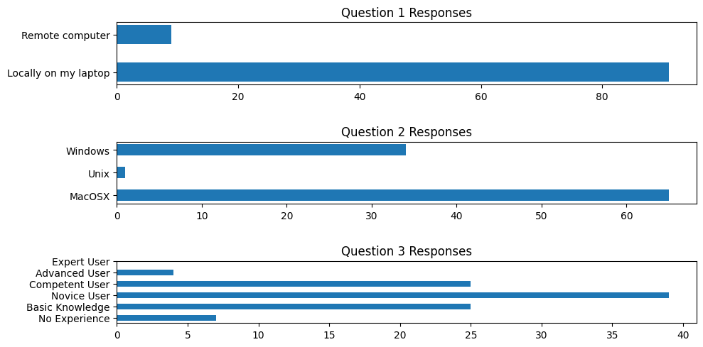
Results of entry poll are here. And a detailed Stata analysis of these results can be found here
From a simulation#
I planned the first two sessions of this class based on assumptions about your skill levels. One doesn’t always have the luxury of real data. But decisions must be made.
Show code cell source
# House cleaning
import matplotlib.pyplot as plt
import numpy as np

fig, axs = plt.subplots(3, 1, figsize=(10, 5))

# Adjust the height of bars here
bar_height = 0.5

#
# Set the random seed for reproducibility
np.random.seed(0)

# Simulate responses for question 1 (Stata usage location)
q1_responses = np.random.choice(['Locally on my laptop', 'Remote computer'], 100, p=[0.9, 0.1])

# Simulate responses for question 2 (Operating system)
q2_responses = np.random.choice(['MacOSX', 'Unix', 'Windows'], 100, p=[0.67, 0.01, 0.32])

# Simulate responses for question 3 (Experience level)
# Assuming a mean experience level of 2 (Novice User) with a standard deviation of 1
q3_responses = np.random.normal(loc=2, scale=1, size=100)
# Ensure the experience level is within the 0 to 5 range and round to the nearest integer
q3_responses = np.clip(q3_responses, 0, 5).round().astype(int)

# Question 1
q1_values, q1_counts = np.unique(q1_responses, return_counts=True)
axs[0].barh(q1_values, q1_counts, height=bar_height)
axs[0].set_title('Question 1 Responses')
axs[0].set_xlabel(' ') # Number of Responses

# Question 2
q2_values, q2_counts = np.unique(q2_responses, return_counts=True)
axs[1].barh(q2_values, q2_counts, height=bar_height)
axs[1].set_title('Question 2 Responses')

# Question 3
q3_values, q3_counts = np.unique(q3_responses, return_counts=True)
axs[2].barh(q3_values, q3_counts, height=bar_height)
axs[2].set_title('Question 3 Responses')
axs[2].set_ylabel(' ') # Experience Level
axs[2].set_yticks(range(6))
axs[2].set_yticklabels(['No Experience', 'Basic Knowledge', 'Novice User', 'Competent User', 'Advanced User', 'Expert User'])

plt.tight_layout()
plt.show()
Show code cell output
From zoom poll#
Show code cell source
import pandas as pd
import matplotlib.pyplot as plt
from IPython.display import Image, display
import io

# Load the CSV file to examine its structure
url = 'https://raw.githubusercontent.com/jhustata/basic/main/entry_poll.csv'
data_path = '~/documents/github/stataone/entry_poll.csv'
survey_data = pd.read_csv(data_path)

# Data processing for visualization

# Question 1: Stata usage location
q1_data = survey_data['How will you use Stata from 03/26/2024-05/17/2024?']
q1_counts = q1_data.value_counts()

# Question 2: Operating system usage, handling multiple selections
# Splitting the responses on ';' and flattening the list
q2_data_split = survey_data['What operating system will you use locally or remotely?'].str.split(';').explode()
q2_counts = q2_data_split.str.strip().value_counts()

# Question 3: Experience level, translating text responses into numeric levels
experience_mapping = {
    'No Experience.': 0,
    'Basic Knowledge.': 1,
    'Novice User.': 2,
    'Competent User.': 3,
    'Advanced User.': 4,
    'Expert User.': 5
}

# Extract the first part of each response to map to the numeric values
q3_data_mapped = survey_data['Do you have any experience using Stata, SAS, R, Python, or any other statistical software?']\
                    .str.split('.').str[0] + '.'
q3_data_numeric = q3_data_mapped.map(experience_mapping)
q3_counts = q3_data_numeric.value_counts().sort_index()

# Visualization
fig, axs = plt.subplots(3, 1, figsize=(10, 12))

bar_height = 0.5

# Question 1
axs[0].barh(q1_counts.index, q1_counts.values, height=bar_height)
axs[0].set_title('Question 1 Responses: Stata Usage Location')
axs[0].set_xlabel('Number of Responses')

# Question 2
axs[1].barh(q2_counts.index, q2_counts.values, height=bar_height)
axs[1].set_title('Question 2 Responses: Operating System Used')

# Question 3
axs[2].barh(q3_counts.index, q3_counts.values, height=bar_height)
axs[2].set_title('Question 3 Responses: Experience Level')
axs[2].set_xlabel('Number of Responses')
axs[2].set_yticks(range(6))
axs[2].set_yticklabels(['No Experience', 'Basic Knowledge', 'Novice User', 'Competent User', 'Advanced User', 'Expert User'])

plt.tight_layout()

# Instead of plt.show(), save the plot to a BytesIO object and display it inline
buf = io.BytesIO()
plt.savefig(buf, format='png', bbox_inches='tight')
buf.seek(0)
display(Image(buf.getvalue()))

# It's important to close the plt object to free up memory
plt.close(fig)
Show code cell output
---------------------------------------------------------------------------
FileNotFoundError                         Traceback (most recent call last)
Cell In[2], line 9
      7 url = 'https://raw.githubusercontent.com/jhustata/basic/main/entry_poll.csv'
      8 data_path = '~/documents/github/stataone/entry_poll.csv'
----> 9 survey_data = pd.read_csv(data_path)
     11 # Data processing for visualization
     12
     13 # Question 1: Stata usage location
     14 q1_data = survey_data['How will you use Stata from 03/26/2024-05/17/2024?']

File ~/Documents/Rhythm/myenv/lib/python3.12/site-packages/pandas/io/parsers/readers.py:1026, in read_csv(filepath_or_buffer, sep, delimiter, header, names, index_col, usecols, dtype, engine, converters, true_values, false_values, skipinitialspace, skiprows, skipfooter, nrows, na_values, keep_default_na, na_filter, verbose, skip_blank_lines, parse_dates, infer_datetime_format, keep_date_col, date_parser, date_format, dayfirst, cache_dates, iterator, chunksize, compression, thousands, decimal, lineterminator, quotechar, quoting, doublequote, escapechar, comment, encoding, encoding_errors, dialect, on_bad_lines, delim_whitespace, low_memory, memory_map, float_precision, storage_options, dtype_backend)
   1013 kwds_defaults = _refine_defaults_read(
   1014     dialect,
   1015     delimiter,
   (...)
   1022     dtype_backend=dtype_backend,
   1023 )
   1024 kwds.update(kwds_defaults)
-> 1026 return _read(filepath_or_buffer, kwds)

File ~/Documents/Rhythm/myenv/lib/python3.12/site-packages/pandas/io/parsers/readers.py:620, in _read(filepath_or_buffer, kwds)
    617 _validate_names(kwds.get("names", None))
    619 # Create the parser.
--> 620 parser = TextFileReader(filepath_or_buffer, **kwds)
    622 if chunksize or iterator:
    623     return parser

File ~/Documents/Rhythm/myenv/lib/python3.12/site-packages/pandas/io/parsers/readers.py:1620, in TextFileReader.__init__(self, f, engine, **kwds)
   1617     self.options["has_index_names"] = kwds["has_index_names"]
   1619 self.handles: IOHandles | None = None
-> 1620 self._engine = self._make_engine(f, self.engine)

File ~/Documents/Rhythm/myenv/lib/python3.12/site-packages/pandas/io/parsers/readers.py:1880, in TextFileReader._make_engine(self, f, engine)
   1878     if "b" not in mode:
   1879         mode += "b"
-> 1880 self.handles = get_handle(
   1881     f,
   1882     mode,
   1883     encoding=self.options.get("encoding", None),
   1884     compression=self.options.get("compression", None),
   1885     memory_map=self.options.get("memory_map", False),
   1886     is_text=is_text,
   1887     errors=self.options.get("encoding_errors", "strict"),
   1888     storage_options=self.options.get("storage_options", None),
   1889 )
   1890 assert self.handles is not None
   1891 f = self.handles.handle

File ~/Documents/Rhythm/myenv/lib/python3.12/site-packages/pandas/io/common.py:873, in get_handle(path_or_buf, mode, encoding, compression, memory_map, is_text, errors, storage_options)
    868 elif isinstance(handle, str):
    869     # Check whether the filename is to be opened in binary mode.
    870     # Binary mode does not support 'encoding' and 'newline'.
    871     if ioargs.encoding and "b" not in ioargs.mode:
    872         # Encoding
--> 873         handle = open(
    874             handle,
    875             ioargs.mode,
    876             encoding=ioargs.encoding,
    877             errors=errors,
    878             newline="",
    879         )
    880     else:
    881         # Binary mode
    882         handle = open(handle, ioargs.mode)

FileNotFoundError: [Errno 2] No such file or directory: '/Users/apollo/documents/github/stataone/entry_poll.csv'
GPT-4 Assisted Analysis
GPT-4 produced this analysis in less than a minute. It’s virtually impossible for you to replicate that speed and accuracy, as we’ll see shortly
1.0.3 Understanding Format Specifiers: %9s#
To seamlessly integrate external data into our analysis, let’s start by importing a .csv file directly into Stata. Pay close attention to the variable types discussed in the following section: Understanding Variable Types.
import delimited "https://raw.githubusercontent.com/jhustata/basic/main/entry_poll.csv", clear
For a comprehensive guide on this command, type
help import delimited.Within import_delimited_options, focus on the “varnames” option.
Consider this: if the first row of your dataset includes variable names, how should you proceed?
import delimited "https://raw.githubusercontent.com/jhustata/basic/main/entry_poll.csv", clear varn(1)
For those navigating Stata’s syntax for the first time, remember that any argument following a comma is known as an option. This grants considerable flexibility in data importation, analysis, and output generation. As you develop your programming skills, you’ll learn to offer similar flexibility to your users by incorporating customizable options into your scripts.
Can you challenge yourself to create a bar graph with the imported data? Data can be numeric or string – how do we determine the nature of our dataset?
describe
Identify the format of your variables. Need a hint? Revisit the section 1.2 Overview.
For a thorough analysis using Stata on this dataset, refer to this detailed examination.
Show code cell source
import networkx as nx
import matplotlib.pyplot as plt

G = nx.DiGraph()
G.add_node("1. Root", pos=(-2500, 700))
G.add_node("2. Pentatonic", pos=(-4200, 0))
G.add_node("3. Diatonic", pos=(-2500, -700))
G.add_node("4. Chromatic", pos=(-1000, 0))
G.add_node("5. Temperament", pos=(1500, 0))
G.add_node("6. Expression", pos=(4000, 0))

G.add_edges_from([("1. Root", "4. Chromatic")])
G.add_edges_from([("2. Pentatonic", "4. Chromatic")])
G.add_edges_from([("3. Diatonic", "4. Chromatic")])
G.add_edges_from([("4. Chromatic", "5. Temperament")])
G.add_edges_from([("5. Temperament", "6. Expression")])

pos = nx.get_node_attributes(G, 'pos')
labels = {"4. Chromatic": "4. Agency",
          "1. Root": "1. Tools",
          "2. Pentatonic": "2. Challenges",
          "3. Diatonic": "3. Skills",
          "5. Temperament": "5. Flow",
          "6. Expression": "6. Growth"}  # Added label for "NDI" node in the labels dictionary

# Update color for the "Scenarios" node
node_colors = ["lightblue","lightblue", "lavender", "lightblue", "lightblue", "lightblue"]
# node_colors = ["lightblue","lavender", "lavender", "lightgreen", "lightpink", "lightpink"]
# Suppress the deprecation warning
import warnings
warnings.filterwarnings("ignore", category=DeprecationWarning)

plt.figure(figsize=(10, 8))
nx.draw(G, pos, with_labels=False, node_size=20000, node_color=node_colors, linewidths=2, edge_color='black', style='solid')
nx.draw_networkx_labels(G, pos, labels, font_size=14) # , font_weight='bold'
nx.draw_networkx_edges(G, pos, edge_color='black', style='solid', width=2)
plt.xlim(-5000, 5000)
plt.ylim(-1000, 1000)
plt.axis("off")
plt.show()
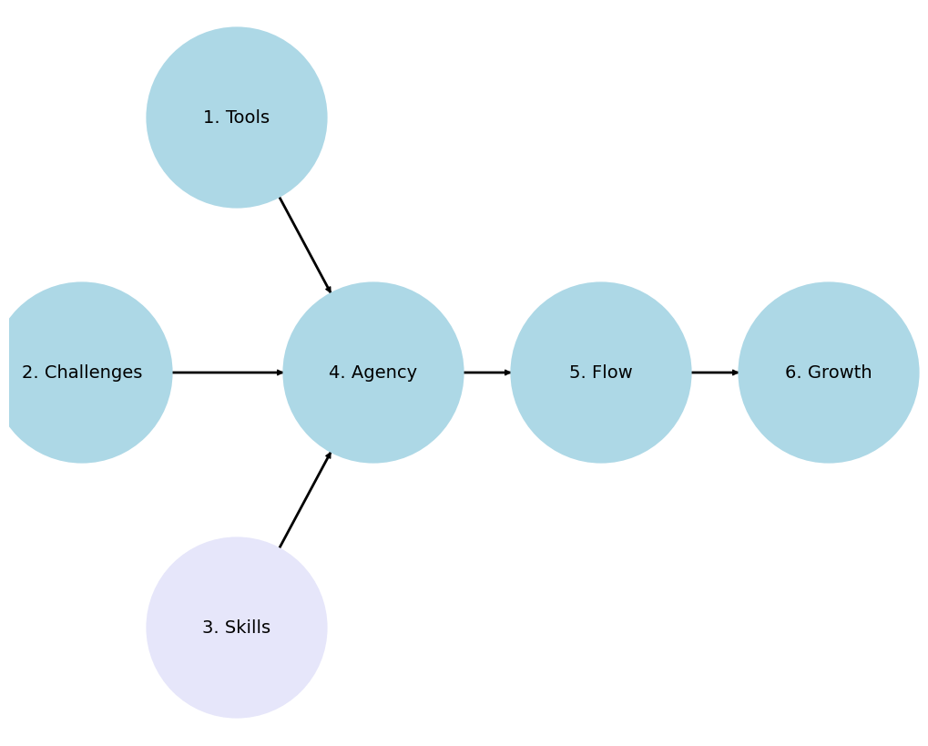
1.1 Philosophy#
In embarking on the journey of mastering Stata for data analysis and statistical programming, we adhere to a philosophy that is both pragmatic and reflective.
1.1.1 Receive & with simplicity#
Tools
Workstation
Remote: Terminal, Safe Desktop
Local: Download to your machine
Installation
Username: 0123456789 (from email)
You’ll use it again even with future purchases
Password:
$3(re+(your choice)Serial number (from purchase)
Perpetual license (expensive)
Subscription
6 months
12 month
Operating system (Windows, Mac, Linux)
Contact Stata if you have other system
Package Stata/MP, Stata/SE, Stata/BE
e.g. Installed the parallel processing version for Mac, ado and help files, PDF documentation, tutorials, and support files. Requires a Stata/MP license
Allow stata to access files in document folder
Courses
340.600 Stata Programming I (Basic)
340.700 Stata Programming II (Intermediate)
340.800 Stata Programming III (Advanced)
Challenges
-
Epi 750 series
Biostats 620 series
Hopkins
Homework
Capstone/Thesis
Biostats 140.624
Real-World
-
Demographic
Questionnaire
Nutrition
Lab
Exam
Outcomes (30-year followup)
Mortality
Kidney failure
National Databases
Clinical Studies
Longitudinal Cohorts
-
-
1.1.2 Know & be reverent#
Skills
Analytical Thinking: You are encouraged to not just learn Stata syntax but to understand the data you are working with. Stata is not just a tool but a gateway to meaningful insights. This class assumes that you have received some training in epidemiology and biostatistics and will not be emphasizing any of these points.
Data Management Mastery: Knowing how to efficiently clean, manipulate, and prepare data is sacred in the realm of statistical analysis. Treat each dataset as a unique puzzle that tells a story. I’ve two datasets that have the same information, but in different formats. From a technical perspective, there might be nuanced differences in the challenges you’ll encounter while using one dataset compared with another.
Statistical Techniques: A reverent understanding of the statistical methods behind the commands is crucial but beyond the scope of this class. For instance, we will not discuss the relative merits of three approaches to survival analysis: non-parametric, semi-parametric, and parametric. This class assumes you know why and when to use each method. But we will provide you with the tools to do so efficiently.
Agency
Self-directed Learning: We hope you appreciate the value of exploration beyond the classroom. The most profound learning occurs through tackling real-world data challenges.
Community Contribution: Please engage with our new Stata-focused community, share knowledge, ask questions, and contribute solutions. Respect for the community’s collective wisdom and the software’s capabilities should guide your interactions.
1.1.3 Do & on time#
Flow
Start with the Basics: This class, as it’s name suggests, emphasizes the importance of a strong foundation. Understanding the
basicsthoroughly ensures smoother progression tointermediateandadvancedtopics.Practical Applications: If you need a real-world dataset (e.g. NHANES) for your Biostats 140.624 project, we’d be happy to facilitate you and help curate it for you. Hopefully this will foster a deeper understanding and appreciation of Stata’s power.
Iterative Learning: Please use an iterative approach to all your labs and homeworks. The first attempt doesn’t have to be perfect; learning comes from refinement and persistence.
Growth
Feedback Loops: Constructive feedback is sacred. So we are offering an open environment where feedback is given and received, to promote continuous improvement and learning.
Skill Expansion: The course is structured to progressively challenge you with more complex problems and datasets. Growth in the realm of Stata Programming, and in any aspect of life in general, is about matching challenges with skills. But gradually and systematically increasing the challenges we present to you, and by offering you prompt feedback on your performance, we believe we’ll nurture an environemnt that ensures growth in your skills.
Lifelong Learning: And remember that learning Stata, like any other skill, is a journey without an end. The landscape of data analysis is always evolving, and so should your skills and understanding. This is partly what motivated our new Stata-focused community as well as our general analytic community that aims to discuss topics at the interface of Stata, R, Python, AI, code, version control, automation, open science, etc.
1.2 Overview 🦀#
Ceci n’est pas une crabe
Show code cell source
import networkx as nx
import matplotlib.pyplot as plt
#import numpy as np
#import sklearn as skl
#

#plt.figure(figsize=[2, 2])
G = nx.DiGraph()
G.add_node("user",  pos = (550,500) )
G.add_node("system",  pos = (-550,500) )
G.add_node("program",  pos = (-2000, 960) )
G.add_node("syntax",  pos = (2000, 950) )
G.add_node("ado", pos = (-3000, 550) )
G.add_node("do", pos = (3000, 550) )
G.add_node("command", pos = (-1900, 150) )
G.add_node("queue", pos = (1900, 150) )
G.add_node("results", pos = (0,0))
G.add_node("dta", pos = (0, -475))
G.add_node("log", pos = (-1900, -475))
G.add_node("excel", pos = (-4000, -475))
G.add_node("word", pos = (1900, -475))
G.add_node("html", pos = (4000, -475))
G.add_node("publish", pos = (0, -950))
G.add_edges_from([ ("program","ado"), ("syntax", "do")])
G.add_edges_from([("ado", "command"), ("do", "queue") ])
G.add_edges_from([("command", "results"), ("queue", "results"),("results","excel"),("results","word"),("results","html")])
G.add_edges_from([("results","dta"),("results","log")])
G.add_edges_from([("dta","publish"),("log","publish"),("excel","publish"),("word","publish"),("html","publish")])
nx.draw(G,
        nx.get_node_attributes(G, 'pos'),
        with_labels=True,
        font_weight='bold',
        node_size = 4500,
        node_color = "lightblue",
        linewidths = 3)
ax= plt.gca()
ax.collections[0].set_edgecolor("#000000")
ax.set_xlim([-5000, 5000])
ax.set_ylim([-1000, 1000])
plt.show()
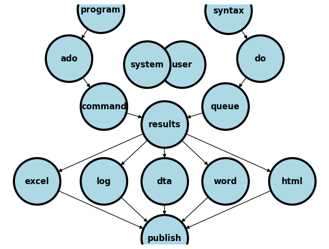
1.2.1 User vs. system#
We are going to distinguish between two fundamental perspectives in this class:
System
Native (built-in stata application, support files,
.adofiles)If you type
which helpinto your command window you get something like:/Applications/Stata/ado/base/h/help.ado
Third-party (typically
.adofiles)When I type
which table1_fenaI get/Applications/Stata/ado/base/t/table1_fena.ado
Your
.adofiles (you’ll learn to write & install your own programs)Since you don’t have
table1_fena.adoinstalled you’ll getcommand table1_fena not found as either built-in or ado-file
User
Known
Instructor
Teaching assistants
Students
Collaborators
Unknown
Anticipate (emphathize with different kinds of users)
Share code (on GitHub, for instance)
Care (user-friendly, annotated code)
The system is the Stata application and its a simple noun. It is not STATA, which gives the impression of being an acronym. I presume you’ve all installed Stata onto your local machines. If not I presume you’ll be doing so very soon or you will be remotely accessing it. The user includes you, me, the teaching assistants, collaborators, or strangers.
As a user, you will or have already downloaded and installed a system of programs, mostly ado-files, which form the foundation of all the commands you will be using in Stata. These are the native Stata system files.
But soon you will begin to write your own Stata programs or .ado files and install them into the system folders (as I’ve done with table1_fena.ado). Then, it will be helpful to think of your role as part of the system. In your new role as system, it will be helpful to anticipate the needs of the known and unknown future users of your program. This will call for empathy (anticipating user needs), sharing (your code with others), and caring (that its user-friendly).
1.2.2 Interface#
Installation
Local
MacOSX
Unix
Windows
Remote
Desktop
Windows
Cluster
Unix/Terminal
Local
-
file
edit
view
data
graphics
statistics
user
window
command ⌘ 1
results ⌘ 2
history ⌘ 3
variables ⌘ 4
properties ⌘ 5
graph ⌘ 6
viewer ⌘ 7
editor ⌘ 8
do-file ⌘ 9
manager ⌘ 10
help
Command
The very first
validword you type into the command window or on a line of code in a do fileRendered blue in color if its a native Stata command (on my machine)
A third-party program/command appears white and may not work if you share your do file with others
Your collaborators, TAs, and instructors must be warned about the need to first install such third-party programs
Syntax
The arrangement of words after a Stata command
Create well-formed instructions in Stata (i.e., the syntax of Stata)
Other terms or synonyms include code, Stata code, code snippet.
Input
Menu (see above: a menu-driven task outputs command and syntax in the results window)
do files (Stata script with a sequence of commands; you can copy & paste some from the results window)
ado files (Stata script with a program or a series of programs for specific or general tasks)
-
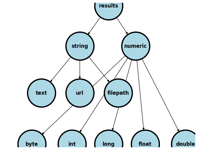
1.2.3 Variable types#
Output/Results
String
text (e.g.,
str49below = string of 49 characters including spaces)The median age in this population is 40 years old
url
https://www.stata-press.com/data/r8
filepath
/users/d/desktop
Numeric (types by range)
integer
byte: \(-127\) to \(100\)int: \(-32767\) to \(32740\)long: \(\pm 2\) billion
decimal
float: \(\pm 10^{38}\) billiondouble: \(\pm 10^{307}\) billion
Show code cell source
import networkx as nx
import matplotlib.pyplot as plt

#plt.figure(figsize=[2, 2])
G = nx.DiGraph()
G.add_node("results", pos = (500,960))
G.add_node("string", pos = (-1000, 400) )
G.add_node("numeric", pos = (1900, 400) )
G.add_node("text", pos = (-3000, -250) )
G.add_node("url", pos = (-1000, -250) )
G.add_node("filepath", pos = (1000, -250) )
G.add_node("long", pos = (500, -960))
G.add_node("int", pos = (-1400, -960))
G.add_node("byte", pos = (-3500, -960))
G.add_node("float", pos = (2400, -960))
G.add_node("double", pos = (4500, -960))
G.add_edges_from([ ("results","string")])
G.add_edges_from([("string", "text"),("string", "url") ,("string", "filepath")])
G.add_edges_from([("numeric","byte"),("numeric","float"),("numeric","double"),("numeric","int")])
G.add_edges_from([("numeric","long"),("results","numeric")])

nx.draw(G,
        nx.get_node_attributes(G, 'pos'),
        with_labels=True,
        font_weight='bold',
        node_size = 4500,
        node_color = "lightblue",
        linewidths = 3)
ax= plt.gca()
ax.collections[0].set_edgecolor("#000000")
ax.set_xlim([-5000, 5000])
ax.set_ylim([-1000, 1000])
plt.show()
1.2.4 Final products#
Embed
Results window
Graph
File: excel, log, dta, word, html, etc.
Publish/Markup
Self (e.g., GitHub)
Journal (e.g. JAMA)
Commercial (e.g. Pfizer Ad)
Let’s use a simple example to illustrate some of the terms we’ve introduced:
Menu
file > example datasets > lifeexp.dta > use
sysuse lifeexp.dtawebuse lifeexp.dtause https://www.stata-press.com/data/r8/lifeexp.dta
do file
Importing data
Exploring data
Analyzing data
Outputing results
ado file
basis of Stata commands
etc.
In the
Basicclass we’ll emphasize .log file and .xlsx as our key output productsHowever, we’ll demonstrate how to output .dta, .docx, .html as well
1.3 Commands#
Let’s instruct Stata to import some data:
webuse lifeexp, clear
. webuse lifeexp, clear
(Life expectancy, 1998)

.
The results window has some output informing us that we’ve imported Life expectancy data from 1998. Now let’s explore these imported data:
display c(N)
display c(k)
describe
. display c(N)
68

. display c(k)
6

. describe

Contains data from https://www.stata-press.com/data/r18/lifeexp.dta
Observations:            68                  Life expectancy, 1998
Variables:                6                  26 Mar 2022 09:40
(_dta has notes)

Variable      Storage   Display    Value
name            type    format     label      Variable label

region          byte    %16.0g     region     Region
country         str28   %28s                  Country
popgrowth       float   %9.0g               * Avg. annual % growth
lexp            byte    %9.0g               * Life expectancy at birth
gnppc           float   %9.0g               * GNP per capita
safewater       byte    %9.0g               * Safe water
* indicated variables have	notes

Sorted by:

.
By now you should be quick to point out that display is a command. To better understand what this command does, you can type help display in the command window. If you do so, you’ll learn the following:
[P] display	--	Display strings and values of scalar expressions
			(View complete PDF manual entry)
In our earlier discussion, we covered two main types of data output in Stata: string and numeric values. The display command is used to show these values, formatted according to the syntax you specify.
Data outputs generally have two main features:
Name: For example,
c(N)refers to the number of observations, andc(k)refers to the number of variables.Content: This is the actual value associated with the name, such as the actual number of observations and variables.
These are examples of what are known as macros. Specifically, they are system-defined macros. We will also explore user-defined macros, which you can create yourself, in our next session.
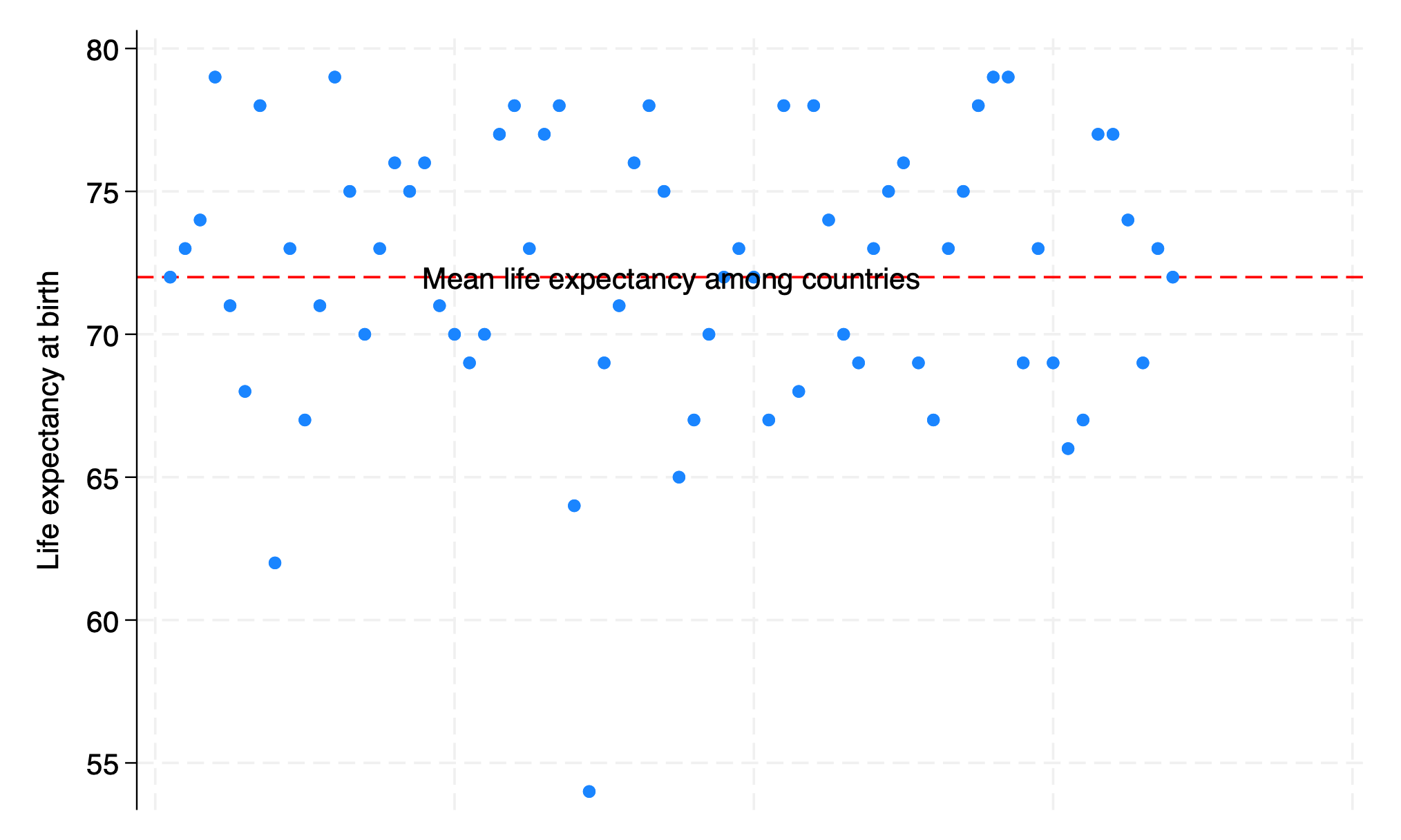
Now, let’s practice some basic data analysis with our imported dataset to understand more about Stata syntax and outputs. We’ll go through each line of code and add explanations:
webuse lifeexp, clear
encode country, gen(Country)
twoway scatter lexp Country, xscale(off)
graph export lexp_bycountry.png, replace
Loading the Data:
webuse lifeexp, clearThis command loads a dataset named
lifeexpinto Stata. Theclearoption is used to ensure that any previously loaded data is removed from memory, making room for this new dataset.
Creating a New Variable:
encode country, gen(Country)Here, we’re taking the
countryvariable, which contains country names, and converting it into a new numeric variable namedCountry. This process assigns a unique number to each country name, making it easier to work with in statistical analyses.
Generating a Scatter Plot:
twoway scatter lexp Country, xscale(off)This line of code creates a scatter plot with life expectancy (
lexp) on one axis and the newly createdCountryvariable on the other. Thexscale(off)part means we’re not scaling the x-axis, keeping it in its original state for clarity.
Exporting the Graph:
graph export lexp_bycountry.png, replaceFinally, this command saves the scatter plot as an image file named
lexp_bycountry.png. Thereplaceoption allows the file to be overwritten if it already exists, ensuring your latest graph is saved.
By following these steps, you’re performing a basic yet insightful analysis of your data, exploring the relationship between countries and life expectancy. This hands-on approach will help you become more familiar with Stata’s syntax and how to interpret the outputs of your analyses.
. webuse lifeexp, clear
(Life expectancy, 1998)

. encode country, gen(Country)

. twoway scatter lexp Country, xscale(off)

. graph export lexp_bycountry.png, replace
file /Users/d/Desktop/lexp_bycountry.png saved as PNG format

.
1.4 Syntax#
A few commands are useful on their own:
chelp
pwd
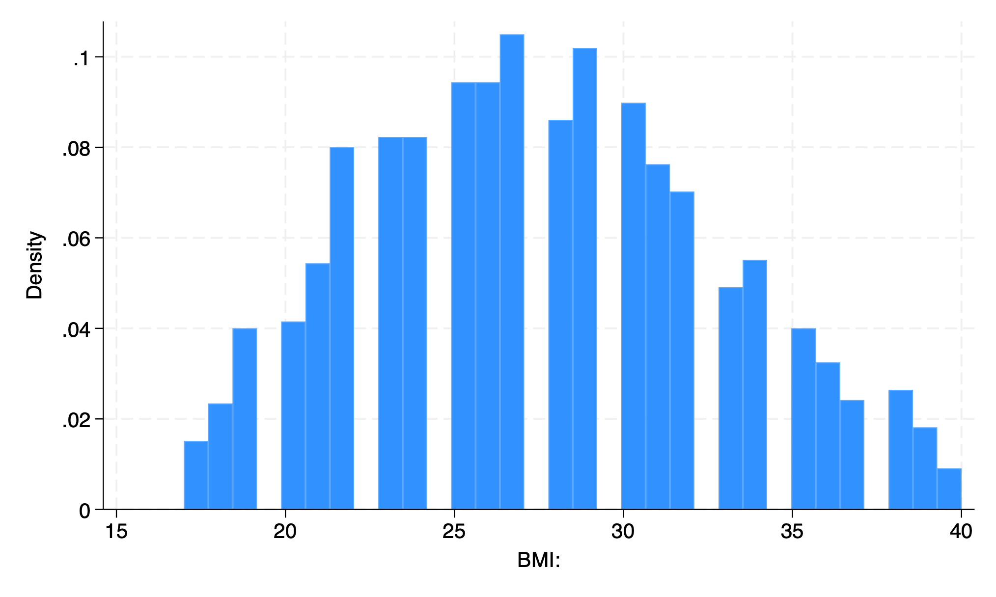
To name but a few. But the vast majority of commands will only work in context of the appropriate syntax. In this example below, the command clear is useful on its own. But set only becomes useful with additional syntax. Here we have obs 1000, instructing Stata to create an empty dataset with 1000 observations. The command generate with syntax bmi=rnormal(28,5) then instructs Stata to create a new variable bmi in a simulation of a random sampling process with replacement, 1000 times over, from a population with mean bmi of 28 and standard deviation of 5. Stata is then instructed to create a histogram of these simulated bmi sample and save the figure as a .PNG image. Hopefully this clarifies what a Stata command is and what syntax is. Together these make up Stata code.
 clear
 set obs 1000
 generate bmi=rnormal(28,5)
 histogram bmi, normal
 graph export bmi.png, replace
.  clear

.  set obs 1000
Number of observations (_N) was 0, now 1,000.

.  generate bmi=rnormal(28,5)

.  histogram bmi, normal
(bin=29, start=13.457429, width=.99248317)

.  graph export bmi.png, replace
file /Users/d/Desktop/bmi.png saved	as	PNG	format

.
end of do-file

.
In the above example the very first valid word is a command and is rendered blue on my machine but purple in this book. If you type any random word that has no corresponding ado-file, you’ll get an error message. Notice also that since its not a native Stata command, it appears black (or white), but not purple.
myfirstprogram
. myfirstprogram
command myfirstprogram is unrecognized
r(199);

.
The words that come after the command might be further commands or subcommands. If so, they’ll also be rendered blue on my machine. The ones that appear in white or black (dark or light mode) are either third-party programs/commands or they are part of the Stata syntax. By the end of next week you’ll be writing your first program (which becomes a Stata command). And by week three you’ll be adding requirements for syntax, which introduces user-defined input.
1.5 Lab#
data: transplants.dta
Please use this lab as an opportunity to review the course material and prepare yourself for the homework 1 & 2 questions. An answer key will be on Friday April 5, 2024. Question 14 will prepare you for homework 1.
Start Stata and open your do-file editor.
You will now write your first do-file following the guidelines given in lecture1.do.
We want to load
transplants.dta. You may do so directly from the class website using a URL. Alternatively, you may download this file onto your local machine. In the latter case, let’s check your working directory. See the bottom left side of the console (the main Stata window). You may also typepwdon the console. Is it where yourtransplants.dtais located? If not, use one of these two methods:
a) Next time, launch Stata by double-clicking on transplants.dta.
b) Type cd c:\your\actual\path (windows OS) on the console (NOT in your do file). In class and on my Mac OS my directory was /Users/d/desktop
Now let’s get back to your do file. Load
transplants.dta(double-click on the file or typeuse transplants.dta, clear)How many observations does the dataset have?
How many adults (age>18) does the dataset have?
How many observations have missing bmi?
Generate a new variable called agecat. The value of agecat is 1 for patients younger than 18, 2 for those from 18 to 65, and 3 for those older than 65.
What are the means of age and bmi?
Now preserve your dataset (type
help preserveto learn more).Drop all patients who are younger than 18 or older than 65, or have missing value for age.
Again, what are the means of age and bmi? restore the dataset. Yet again, what are the means of age and bmi?
What happened? Leave a comment on your do-file explaining what you just did. Remember, your homework (and all other) .do file scripts should have 1-3 comments per block of code. Do not use your comments/annotation to define the Stata commands you’ve used. Thats what the
helpcommand is for. Instead, give yourself or a reader some context.Lab 1 is almost over. Let Stata say “that was easy!”
The last bit. Close your log file. Never forget to close log files! If you hadn’t created a log file, this is a reminder to do so.
You have all your commands so far in your do file, right? Run your entire do file and make sure your do file does exactly the same thing.
1.6 Homework#
Your week 1 homework is very simple:
Write a .do file which imports data from hw1.tx
Name it
hw1.lastname.firstname.doIt should create a .log file called
hw1.lastname.firstname.logMake sure your log file displays only the output of interest
But do not submit your log file as part of the assignment
Evaluation will be based on the .log file produced when we run your script on our machines
Question:
Print the following sentence: Question 1: There are xxxx records in the dataset. The xxxx should be replaced with the actual number of records in the dataset.
If you are not sure where the backquote is, its to the left of “1” on most keyboards. The forwardquote is to the left of “return” on a Mac. You need to get familiar with these quotes, since they’ll be used to specify “macros” throughout this class and your programming life. While using a .do file, the use of a back quote will automatically generate a forward quote to enclose the specified macro as seen below.
di `c(N)'
