4. Basic file management, Programming options

• Basic file management

  • 4.1 Creating files

  • 4.2 Merging files

• Programming

  • 4.3 Adding options

  • 4.4 Postfile in a program

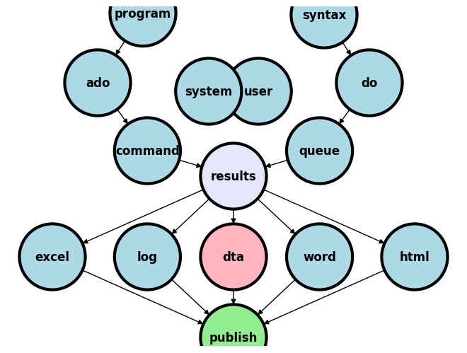
Show code cell source Hide code cell source

import networkx as nx
import matplotlib.pyplot as plt

G = nx.DiGraph()
G.add_node("user", pos=(550, 500))
G.add_node("system", pos=(-550, 500))
G.add_node("program", pos=(-2000, 960))
G.add_node("syntax", pos=(2000, 950))
G.add_node("ado", pos=(-3000, 550))
G.add_node("do", pos=(3000, 550))
G.add_node("command", pos=(-1900, 150))
G.add_node("queue", pos=(1900, 150))
G.add_node("results", pos=(0, 0))
G.add_node("dta", pos=(0, -475))
G.add_node("log", pos=(-1900, -475))
G.add_node("excel", pos=(-4000, -475))
G.add_node("word", pos=(1900, -475))
G.add_node("html", pos=(4000, -475))
G.add_node("publish", pos=(0, -950))
G.add_edges_from([("program", "ado"), ("syntax", "do")])
G.add_edges_from([("ado", "command"), ("do", "queue")])
G.add_edges_from([("command", "results"), ("queue", "results"), ("results", "excel"), ("results", "word"), ("results", "html")])
G.add_edges_from([("results", "dta"), ("results", "log")])
G.add_edges_from([("dta", "publish"), ("log", "publish"), ("excel", "publish"), ("word", "publish"), ("html", "publish")])

pos = nx.get_node_attributes(G, 'pos')
node_colors = ["lightblue" if node not in ["results", "dta", "publish"] else "lightpink" if node == "dta" else "lavender" if node == "results" else "lightgreen" for node in G.nodes()]

nx.draw(G, pos, with_labels=True, font_weight='bold', node_size=4500, node_color=node_colors, linewidths=3)
ax = plt.gca()
ax.collections[0].set_edgecolor("#000000")  # Set edge color to black for better contrast
ax.set_xlim([-5000, 5000])
ax.set_ylim([-1000, 1000])
plt.show()

4.1 Creating files

During our second week had a cursory discussion about the basic files we may output our results into:

• .xlsx

• .log

• .dta

• .docx

• .html

In the Intermediate class we’ve focused mostly on .html, since we’re creating websites to host our content online. In this Basic class we’ve directed our energies at .xlsx and .log, as seen in HW3, which is due today. Its time to revist .dta, which perhaps we didn’t have time to develop in week two. Here’s a link to the notes.

Review of Data Posting and Analysis in Stata

* Clear the previous data and results to ensure a clean workspace.
clear all
cls

* Set up a postfile to store data. This command creates a dataset called output.dta.
* 'a' is a string variable with a maximum length of 80 characters.
* 'b' and 'c' are numeric variables stored as floats.
postfile pp str80 a float(b c) using output.dta, replace

* Post data into the postfile. Each 'post' command adds one observation with three fields.
* 'a' is used as a categorical identifier.
* 'b' and 'c' are quantitative measurements, likely representing some continuous data.
post pp ("1") (24.4) (123)
post pp ("2") (31.5) (164)
post pp ("3") (29.0) (118)

* Close the postfile to finalize changes and prepare the dataset for analysis.
postclose pp

* Load the newly created dataset into memory for further operations.
use output.dta, clear 

* List all observations to verify data integrity and correct input.
list

* Provide a descriptive summary of the dataset, including information on each variable.
describe

We are now in position to apply postfile this to a meaningful example using what we’ve learned so far:

• Variable-type specifiers

• A foreach loop

• Storage of r() values in local macros

postfile to post regression results

postfile pp str80 coef ///
   double(result CIleft CIright pvalue) /// 
   using betas.dta, replace

• Within the script, call our post “pp”

• It will have five variables: a string called coef and doubles (floating-point decimals) called result, CIleft, etc

• The file name on disk will be betas.dta

• If betas.dta exists, replace it

regress bmi gender age
foreach v of varlist gender age {
    //[calculate beta, etc into macros] 
    post pp ("`v'") (`res') (`left') ///
    (`right') (`pvals')
}

foreach v of varlist gender age {
     //[calculate beta, etc into macros] 
     local vlab: variable label `v'
     lincom "`v'" //estimate r() values one variable at a time
     local res: di %3.2f r(estimate)
     local left: di %3.2f r(lb)
     local right: di %3.2f r(ub)
     local pvals: di %3.2f r(p)
     post pp ("`vlab'") (`res') (`left') ///
         (`right') (`pvals')
}

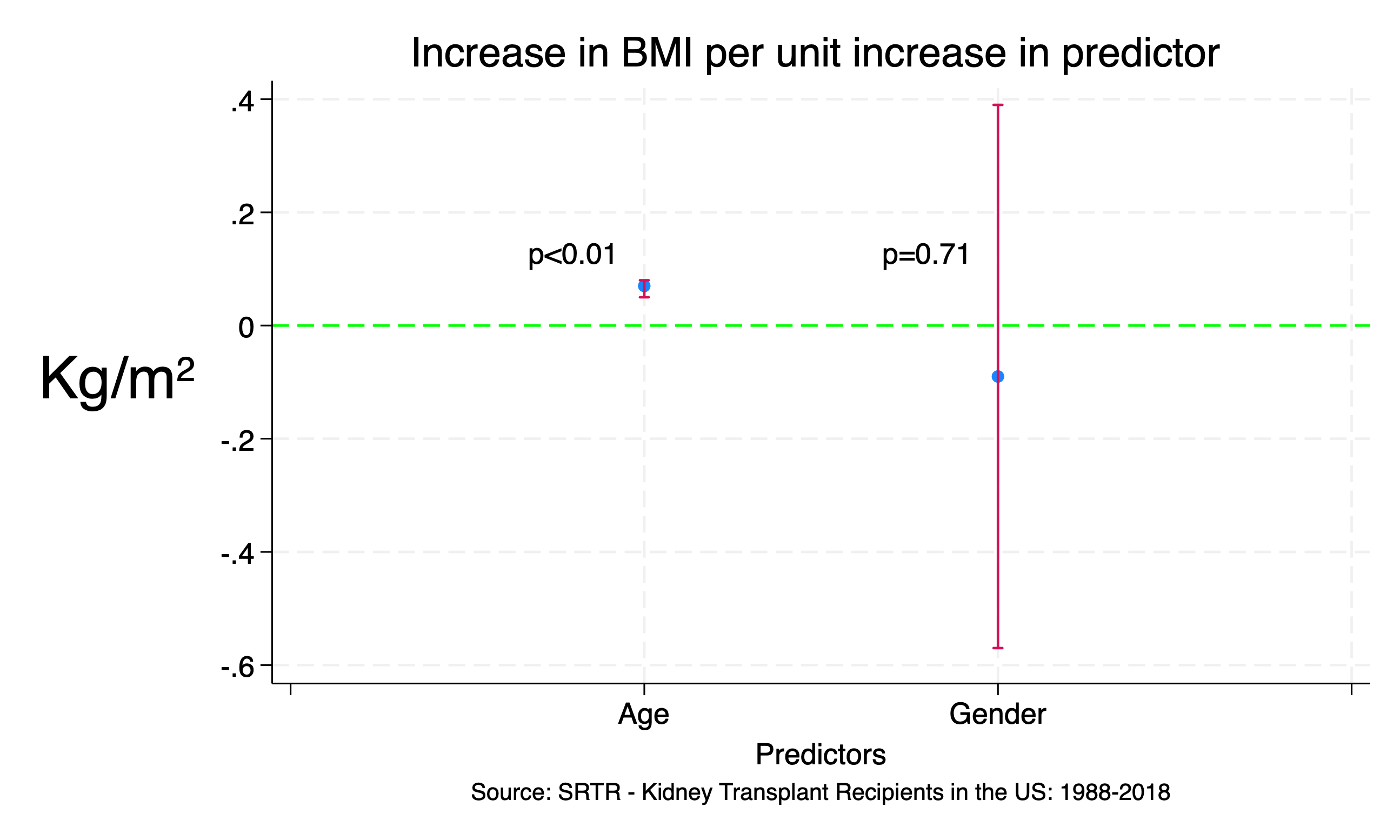
We may use the created betas.dta to visualize our regression output:

use betas, clear 
encode coef, gen(Coef)
twoway (scatter result Coef) ///
 (rcap CIleft CIright Coef ///
, ms(*5) ///
xlab(0(1)3 0 " " 1 "Age" 2 "Gender" 3 " ") ///
xti("Predictors") ///
yti("Kg/m{sup:2}", orientation(horizontal) size(7)) ///
ti("Increase in BMI per unit increase in predictor ") ///
legend(off) ///
yline(0, lc(lime) lp(dash)) ///
text(.13 .8 "p<0.01") ///
text(.13 1.8 "p=0.71") ///
note("Source: SRTR - Kidney Transplant Recipients in the US: 1988-2018", pos(6)) ///
 ) 

• Iterate over variables in a foreach loop

• Calculate beta, 95%CI, pvalue

• Post them to our new dataset

post close pp

• Save and close the file

use betas, clear
list, clean noobs

We can combine this with export excel to write out our own tables in Excel:

use betas, clear 
export excel ///
    coef result CIleft CIright /// 
    using betas_table.xlsx, replace

We can export the results in a publication-friendly format:

gen ci = "(" + string(CIleft, "%3.2f") + ", " + /// 
    string(CIright, "%3.2f") + ")"

export excel coef result ci ///   
    using betas_table2.xlsx, /// 
   replace firstrow(variables)

Let’s improve our output:

label var coef "Variable" 
label var result "Coefficient" 
label var ci "95% CI"
export excel coef result ci ///
    using betas_table3.xlsx, /// 
    replace firstrow(varlabels)

4.2 Merging files

transplants.dta	donors_recipients.dta	donors.dta
fake_id	fake_id	fake_don_id
age	fake_don_id	age_don

Suppose your analytic dataset is transplants.dta and you wish to assess whether donor age is correlated with recipient age in deceased-donor transplants.

Let’s first define our working directory using a macro. (An alternative approach is to download the dataset onto your computer and work in a specific directory with no need for a URL or filepath)

//global url "https://github.com/jhustata/basic/raw/main/"
global url "" //if you are working locally with downloaded datasets

Now let’s import our analytic dataset

use "${url}transplants", clear
lookfor age

We only have the recipients age. So let’s confirm that the variable is in donors.dta:

use "${url}donors", clear
lookfor age

Can we merge transplants.dta with donors.dta to solve this issue?

Simple merge command

use "${url}transplants", clear 
merge 1:1 fake_id ///
    using "${url}donors_recipients"

• We expect each fake_id to appear only once in each dataset (“one-to-one merge”)

• fake_id is the variable that appears in both datasets, letting us link them

• donors_recipients is the dataset that we’re merging with the dataset in memory

tab _merge 

Fancier merge commands

Let’s explore fancier syntax

use "${url}transplants", clear 
merge 1:1 fake_id ///
    using "${url}donors_recipients", ///
    keep(match)

• Only records that appear in both datasets will remain in memory

• Only records that appear in the master dataset only, or in both datasets, will remain in memory

use "${url}transplants", clear 
merge 1:1 fake_id ///
    using "${url}donors_recipients", ///
    gen(mergevar)

• Instead of creating a “system-defined” variable called _merge, lets have a “user-defined” one called mergevar

use "${url}transplants", clear
merge 1:1 fake_id ///
    using donors_recipients, ///
    nogen 

• Don’t create any new variables

• NOTE: if the _merge variable already exists, the _merge command will give an error unless you use gen() or nogen

Two merges in a row

use "${url}transplants", clear
merge 1:1 fake_id ///
    using donors_recipients, ///
    keep(match) nogen 
merge m:1 fake_don_id ///
    using donors, keep(match) nogen ///
    keepusing(age_don)

• Don’t load all variables from the new (using) dataset. Just load age_don

Now lets get back to our original problem: are donor and recipient age correlated?

corr age*

Merging protip

Using merge, keep(match) might drop more records than you expect. If you think all records will match, it’s a good idea to check this assumption

use "${url}transplants", clear merge 1:1 fake_id ///
    using "{url}donors_recipients", ///
    keep(master match)
assert _merge==3

Maybe you don’t expect a perfect match, but you want to make sure nearly all of your records match use transplants, clear

merge 1:1 fake_id ///
    using "${url}donors_recipients", /// 
    keep(master match)
quietly sum _merge
assert r(mean) > 2.98
//99% of records have _merge==3

That’s enough in way of an introduction to the merge command. It will come in handy only in specific projects that have relevant variables in different datasets.

4.3 Adding options

Consider the programs we’ve written over the last two weeks. We discussed:

• program define

• syntax varlist

Now consider this program:

program define opt_demo 
    syntax, [myoption]
    if "`myoption'" != "" {
        disp "You picked the option /// `myoption'"
    } 
    else {
        disp "No option"
    }
end

Invoke the program:

opt_demo
opt_demo, myoption

Let’s look at another example:

program define table1_o
    syntax varlist [if] , [round]

    //set display format
    //if they specified "round", then macro round will equal the word "round"
    //otherwise, it's blank (equals "")
    if "`round'" != "" {  
        local D %1.0f  //macro D will contain the display format
    }
    else {
        local D %3.2f  //set macro D to %3.2f
    }

    disp "Variable" _col(12) "mean(SD)" _col(25) "range"
    foreach v of varlist `varlist' {
        quietly sum `v' `if'
        disp "`v'" _col(12) `D' r(mean) "(" `D' r(sd) ")" _col(25) ///
            `D' r(min) "-" `D' r(max)  //notice we use macro D for format
    }
end

The end-user may now do this:

table1_o age bmi wait_yrs if age<40
table1_o age bmi wait_yrs if age>40, round

Options that take values

program define minmax
    syntax , [min(real 0) max(real 99)] 
    disp "Min: `min'" _col(9) "Max: `max'"
end

minmax
minmax, min(20)
minmax, min(20) max(40)

Another example

program define list_top
    syntax varname, [top(int 10)] 
    preserve
    gsort -`varlist'
    list `varlist' in 1/`top', clean noobs 
end

• Define the program

• Specify that it takes a single variable, and optionally takes the option “top” which is equal to 10 by default

• We’re about to temporarily mess up the dataset, so save a copy so that we don’t mess things up permanently

• Sort in descending order by the variable

• List the top `top’ values of the variable

Updating our table 1 program

Overview table1_nice adds considerable flexibility

Program Structure

• Program Initialization:

  capture program drop table1_nice
  program define table1_nice
  

  This command sequence, as you should be familiar by now, ensures that if table1_nice is already defined, it is removed before defining a new version. This prevents any conflicts with previous definitions.

• Syntax Options:

  syntax varlist [if] , [replace] [precision(int 1)] [title(string)]
  

  Defines the syntax for the program. varlist is mandatory, while if, replace, precision, and title are optional. Each option serves a specific function:

  • if: Allows filtering of data based on conditions.

  • precision: Specifies the number of decimal places for numeric outputs, with a default of 1.

  • title: Allows for a custom title to be displayed at the top of the table.

• Data Preservation and Filtering:

  preserve
  capture keep `if'
  

  The preserve command saves the current dataset state. capture keep attempts to filter the dataset according to the user-defined if condition, suppressing any error if the condition is invalid.

• Display Formatting:

  assert inrange(`precision', 0, 6)
  local pplus = `precision' + 1
  local D %`pplus'.`precision'f
  

  Ensures that the precision falls between 0 and 6. It then adjusts the format string for numeric outputs to match the specified precision.

• Title Display:

  if "`title'" != "" {
      disp "`title'"
  }
  

  Displays the title if one is specified.

• Summary Statistics Table:

  disp "Variable" _col(12) "mean(SD)" _col(25) "range"
  foreach v of varlist `varlist' {
      quietly sum `v' `if'
      disp "`v'" _col(12) `D' r(mean) "(" `D' r(sd) ")" _col(25) `D' r(min) "-" `D' r(max)
  }
  

  Loops through each variable in varlist, calculates summary statistics, and displays them using the specified format. This includes the mean, standard deviation, and range for each variable.

Example Usage

table1_nice age bmi wait_yrs if age>40, precision(2) replace title("Study population")

This command runs table1_nice for variables age, bmi, and wait_yrs for records where age is greater than 40. It uses 2 decimal places for numeric outputs and displays “Study population” as the title.

Conclusion

The table1_nice program offers a customizable approach to data analysis, allowing users to easily generate descriptive statistics tailored to specific research needs.

//combining several of the above techniques into a "table1" program
capture program drop table1_nice
program define table1_nice
    syntax varlist [if] , [replace] [precision(int 1)] [title(string)]
    //if: specify records to include in analysis (optional)
    //precision: # of digits to the right of decimal point (optional, default 1)
    //title: title to display before the table (optional)

    preserve
    capture keep `if' //temporarily drop any records not required

    //set display format
    assert inrange(`precision', 0, 6) //allow 0-6 digits to R of decimal point
    local pplus = `precision' + 1 //first number for formatting code
    local D %`pplus'.`precision'f

    if "`title'" != "" {
        disp "`title'"
    }

    disp "Variable" _col(12) "mean(SD)" _col(25) "range"
    foreach v of varlist `varlist' {
        quietly sum `v' `if'
        disp "`v'" _col(12) `D' r(mean) "(" `D' r(sd) ")" _col(25) ///
            `D' r(min) "-" `D' r(max)  //notice we use macro D for format
    }
end


table1_nice age bmi wait_yrs if age>40, precision(2) replace ///
    title("Study population")

4.4 Postfile in a program

//put it in a program
capture program drop model
program define model
    //takes a varlist of independent (x) variables,
    //a filename to post the data to,
    //and the name of a dependent (y) variable
    syntax varlist, yvar(varname) filename(string)

    regress `yvar' `varlist'

    postfile pp str80 variable double(result CIleft CIright pvalue) ///
        using `filename', replace
    foreach v of varlist `varlist' {
        local res=_b[`v']
        local left=_b[`v']+_se[`v']*invttail(e(df_r),0.975)
        local right=_b[`v']+_se[`v']*invttail(e(df_r),0.025)
        local pval=2*ttail(e(df_r), abs(_b[`v']/_se[`v']))
        post pp ("`v'") (`res') (`left') (`right') (`pval')
    }
    postclose pp
end

• syntax varlist, yvar(varname) filename(string). The program requires a variable list of one or more independent (x) variables for a linear regression, a filename to write the data out to, and a dependent (y) variable

• regress. Run the linear regression

• postfile. Set up the postfile. Write it out to the file name specified by the user

• foreach. Write out the results to our postfile. This part of the code is the same as before we put it into a program

• postclose pp. Close the postfile

use transplants, clear
model age wait_yrs gender rec_hcv, ///
    filename(model_bmi) yvar(bmi)

We may no look at the .dta file we created:

use model_bmi, clear
list, clean noobs

4.5 Lab Session Notes

Key Tasks for This Week

• Review and revise the notes from this week’s sessions. Ensure all information is up-to-date and accurately reflects the discussions and instructions provided.

Essential Skills to Master by Week’s End

By the end of this week, you should be adept at creating programs that not only meet mandatory specifications but also offer enhanced flexibility for end-users. Focus on mastering the following commands and concepts:

1. postfile: Understand how to use this command to efficiently post data to a file buffer. Develop your ability to integrate this function into larger programs where data posting is required.

2. merge: Gain proficiency in merging datasets. Emphasize learning how to align data by key variables and troubleshoot common issues that might occur during the merge process. Your programs should handle merges seamlessly and offer options for handling discrepancies.

3. Syntax and Command Structure:

   • General Syntax: Master the syntax required for your programs: syntax varlist, mandatory options [optional enhancements].

   • Mandatory Options: Ensure your programs can execute essential functions by correctly implementing necessary options.

   • Optional Enhancements: Equip your programs with optional features that provide additional capabilities and customization opportunities to end-users. This approach enhances user satisfaction and program versatility.

Your goal is to develop robust programs that are user-friendly and adaptable to various user needs. Concentrate on these skills to ensure your programs are not only functional but also versatile and user-centric.

4.6 Homework Update

• No Homework This Week (HW4 is Canceled)
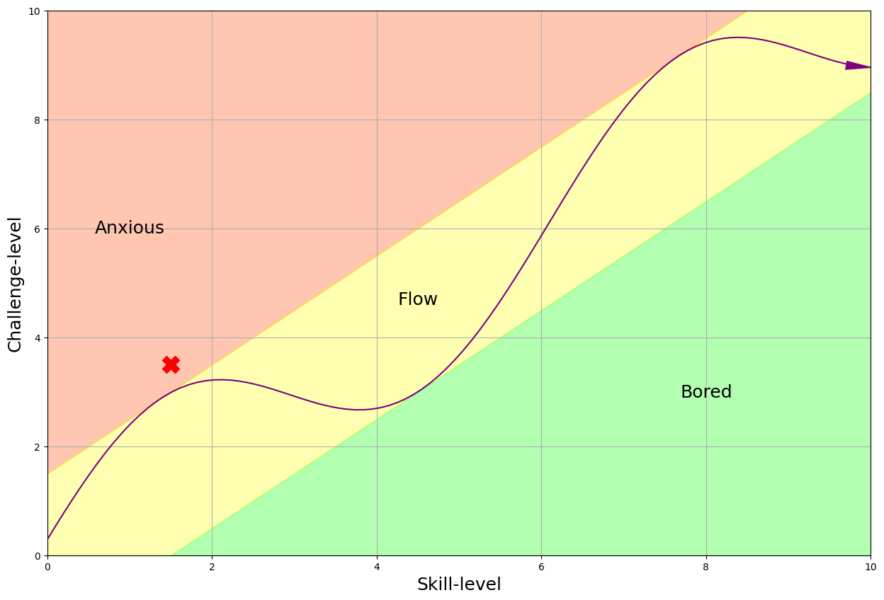
  • We've noticed that Homework 3 was particularly challenging for many of you, with its difficulty (challenge-level 3) leaving many students in the red zone (refer to the figure below). In response to this, we're taking a pause to recalibrate and ensure upcoming assignments better align with the flow zone.
  • This week, take advantage of the break to strengthen your skills:
    • Review the class materials thoroughly.
    • Dive into the GitHub Discussions. You'll find that solutions and helpful insights are frequently shared by your classmates.
    • If you're stuck or need further clarification, don't hesitate to reach out via email. We're here to help!
• Looking Ahead: Homework 5
  • Get ready to jump back into the flow! We will introduce Homework 5 next week, and we're confident you'll find it engaging and appropriately challenging.

Show code cell source Hide code cell source

import matplotlib.pyplot as plt
import numpy as np

# Create data for the skill and challenge levels
skill_levels = np.linspace(0, 10, 100)
challenge_levels = np.linspace(0, 10, 100)

# Define the flow channel boundaries
flow_channel = skill_levels

# Adjust the phase and amplitude of the sinusoid wave
phase = np.pi / 16
amplitude = 1.5
sinusoid = flow_channel + np.sin(skill_levels + phase) * amplitude

# Define the yellow zone boundaries, making it wider
yellow_zone_low = skill_levels - 1.5  # Adjust this value to make the yellow zone wider or narrower
yellow_zone_high = skill_levels + 1.5 # Adjust this value to make the yellow zone wider or narrower

# Plotting
plt.figure(figsize=(15, 10))

# Plot the anxiety and boredom areas
plt.fill_between(skill_levels, yellow_zone_high, 10, color='orangered', alpha=0.3, label='Anxiety Zone', interpolate=True)
plt.fill_between(skill_levels, 0, yellow_zone_low, color='lime', alpha=0.3, label='Boredom Zone', interpolate=True)
plt.fill_between(skill_levels, yellow_zone_low, yellow_zone_high, color='yellow', alpha=0.3, label='Flow Zone', interpolate=True)

# Plot the sinusoid function with the diagonal as its axis
plt.plot(skill_levels, sinusoid, color='purple', linestyle='-')

# Add arrowhead to the sinusoid line
plt.arrow(skill_levels[-2], sinusoid[-2], skill_levels[-1] - skill_levels[-2], sinusoid[-1] - sinusoid[-2],
          color='purple', length_includes_head=True, head_width=0.15, head_length=0.3)

# Add an "X" marker at the specified coordinate
plt.scatter(1.5, 3.5, color='red', s=300, marker='X')

# Set plot labels and title
plt.xlabel('Skill-level', fontsize=18)
plt.ylabel('Challenge-level', rotation='vertical', fontsize=18)

# Set plot limits and grid
plt.xlim(0, 10)
plt.ylim(0, 10)
plt.grid(True)

# Set tick labels
tick_labels = ['0', '2', '4', '6', '8', '10']
plt.xticks(np.linspace(0, 10, 6), tick_labels)
plt.yticks(np.linspace(0, 10, 6), tick_labels)

# Add text annotations to label the areas without shaded background
plt.text(1, 6, 'Anxious', color='black', ha='center', va='center', fontsize=18)
plt.text(4.5, 4.7, 'Flow', color='black', ha='center', va='center', fontsize=18)
plt.text(8, 3, 'Bored', color='black', ha='center', va='center', fontsize=18)

# Display the plot
plt.show()