lab7 Solutions

Please use this lab as an opportunity to review the course material and prepare yourself for hw7. Sample responses to the lab questions are provided below.

global repo https://github.com/jhustata/basic/raw/main/

1. Start Stata, open your do-file editor, write the header, and load transplants.dta.

use "${repo}transplants", clear

2. Get a 10% random sample of the dataset. Specifically, follow these steps. (1) Set a seed number. (2) Generate a variable that includes a random number between 0 and 1 following a uniform distribution. (3) Sort by the random variable. (4) Keep the first 10% observations and drop the rest. (5) Drop the random variable.

   count
   set seed 2024
   gen rdm=runiform()
   sort rdm
   keep if _n<=_N/10
   drop rdm
   count
   
   //alternative
   use transplants, clear
   count
   sample 10
   count
   

3. Clear and reload transplants.dta.

use "${repo}transplants", clear

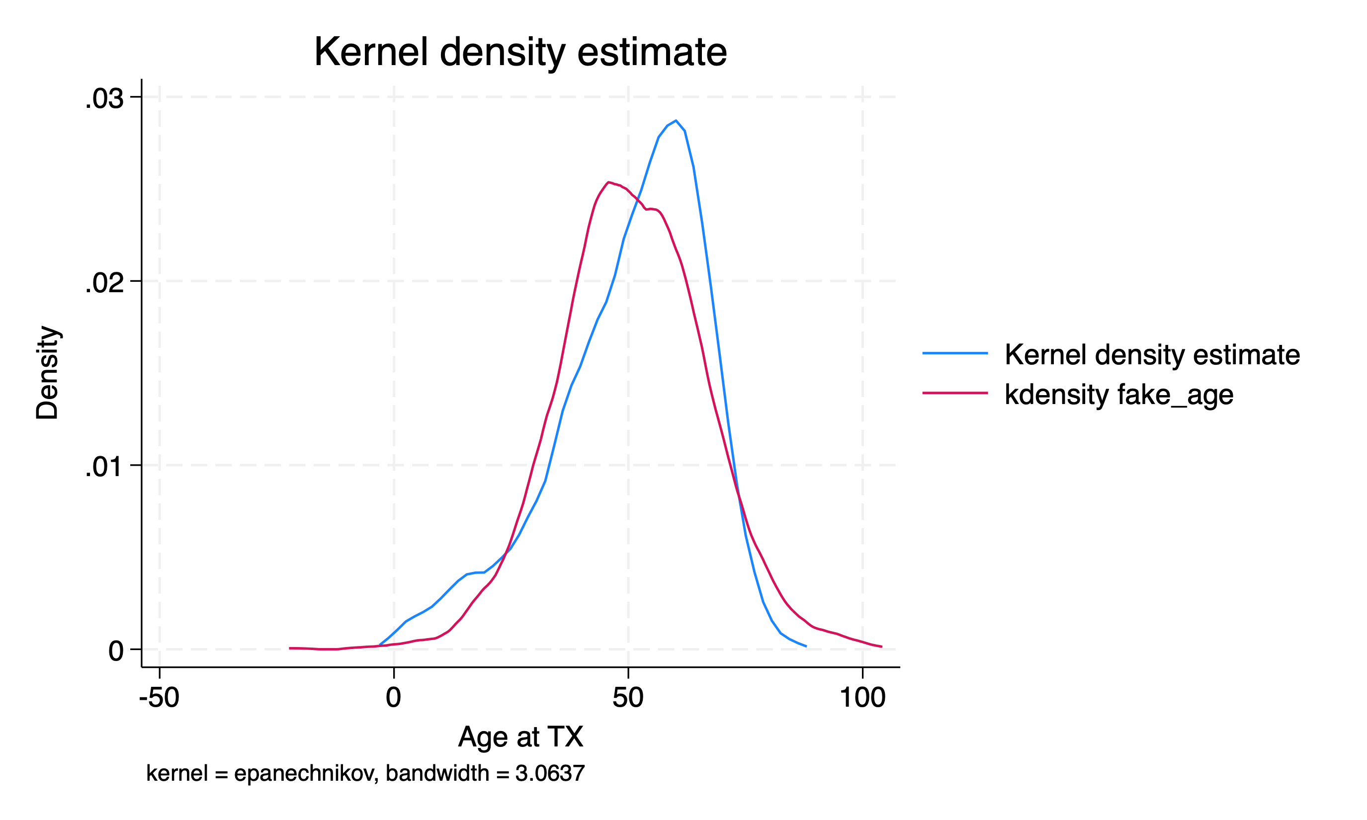
4. Generate a variable called fake_age which is a normally distributed random variable with mean and standard deviation equal to the mean and standard deviation of the actual age variable.

   set seed 123
   sum age age
   g fake_age=rnormal(r(mean), r(sd))
   compare age fake_age
   kdensity age, addplot(kdensity fake_age)
   list fake_id age fake_age in 1/10
   graph export kdensity.png, replace 
   

   

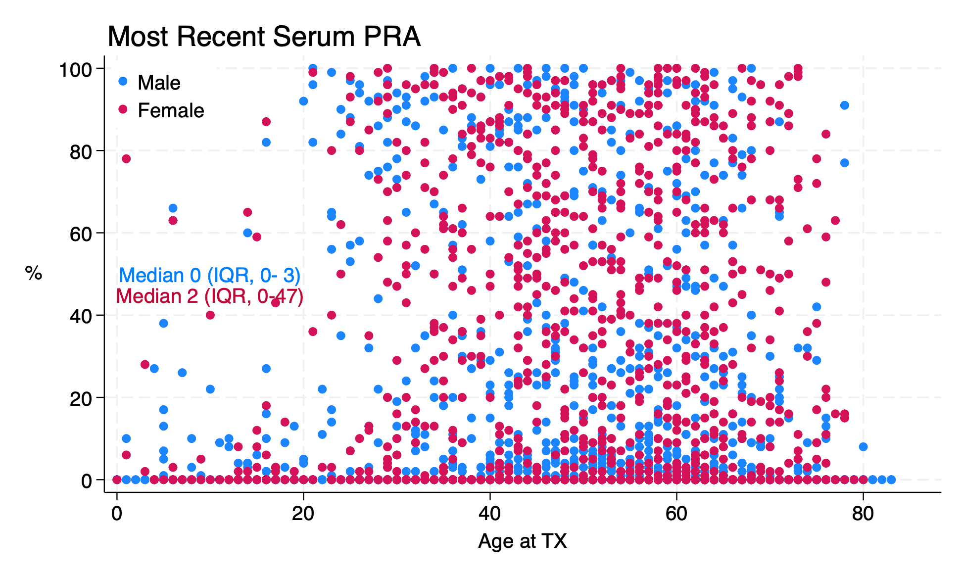
5. Make a scatter plot of peak PRA by age in transplant recipients. Does it look like there’s a relationship between peak PRA and age, and if so, what is the relationship?

use "${repo}transplants", clear 
graph twoway scatter peak_pra age    //full syntax
tw sc peak_pra age                 //abbreviated syntax
   
//explore other twoway options!!  
#delimit ;
forval f=0/1 { ;
	sum peak_pra if gender==`f', d ;
	local m_iqr_`f': di 
       "Median" %2.0f r(p50)
       " (IQR," %2.0f r(p25)
            "-" %2.0f r(p75)
            ")"
			;
} ;
tw (sc peak_pra age if gender==0)
   (sc peak_pra age if gender==1,
       legend(
           on
           ring(0)
           pos(11)
           lab(1 "Male")
           lab(2 "Female")
       )
       ti("Most Recent Serum PRA",pos(11))
       yti("%", orientation(horizontal))
   text(50 10 "`m_iqr_0'",col(midblue))
   text(45 10 "`m_iqr_1'",col(cranberry))
   )
   ;
   #delimit cr
   graph export lab6q5.png, replace 

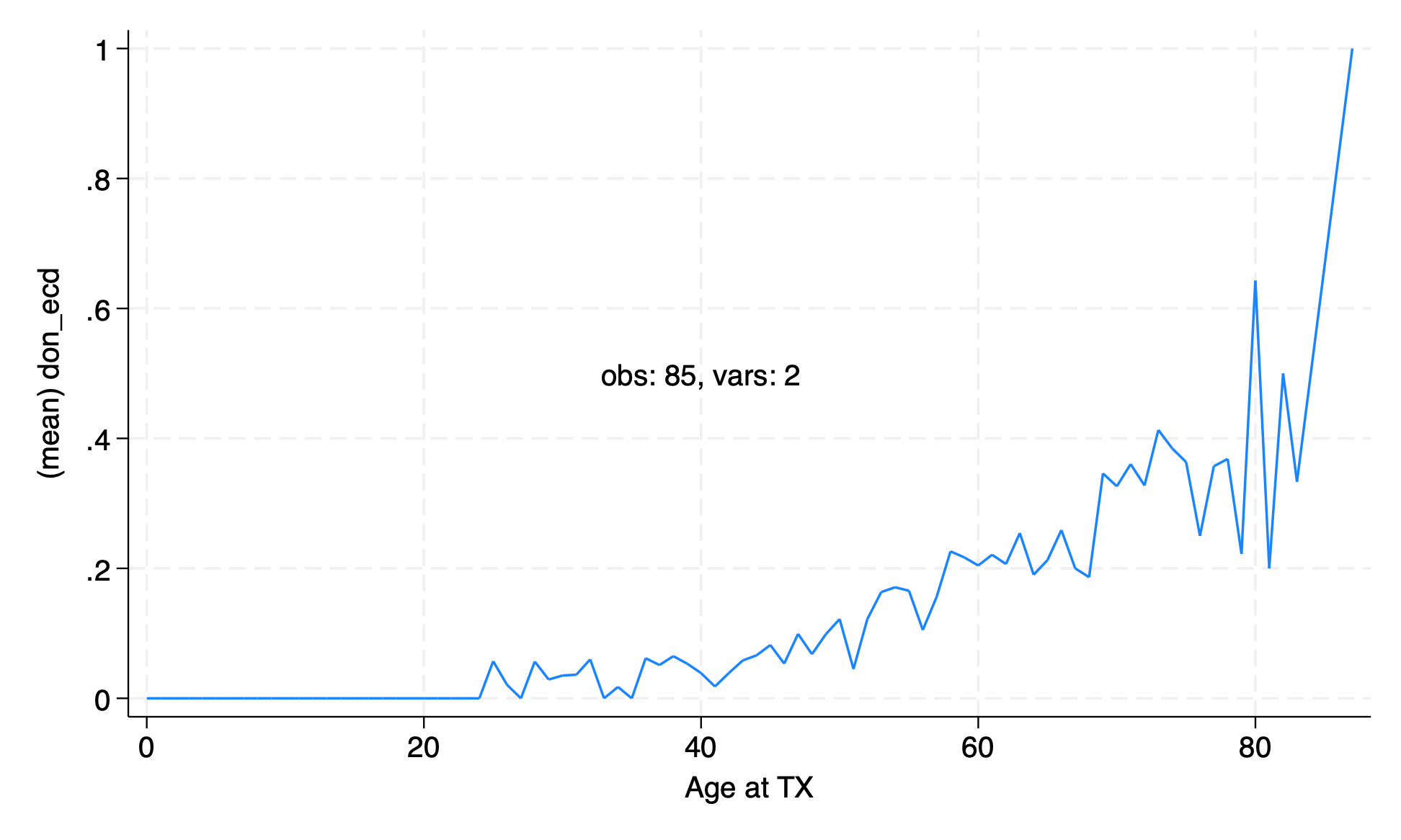
6. The graph of proportion of ECD transplants by age from the lecture was a little messy. Remake the graph with the age rounded to the nearest ten years.

use "${repo}transplants", clear
collapse (mean) don_ecd, by(age)
graph twoway line don_ecd age, text(.5 40 "obs: `c(N)', vars: `c(k)'")
graph export collpasebyage.png,replace
count 
     
//alternative, without messing up the data
if c(N) == r(N) | c(N) == 6000 {
	
use transplants, clear
egen m_don_ecd=mean(don_ecd), by(age)
egen agetag=tag(age)
#delimit ;
line m_don_ecd age if agetag, 
    text(
    .5 40 
    "obs: `c(N)', vars: `c(k)'"
    ) 
    sort ;
#delimi cr
count
graph export lab6q6.png,replace 

}

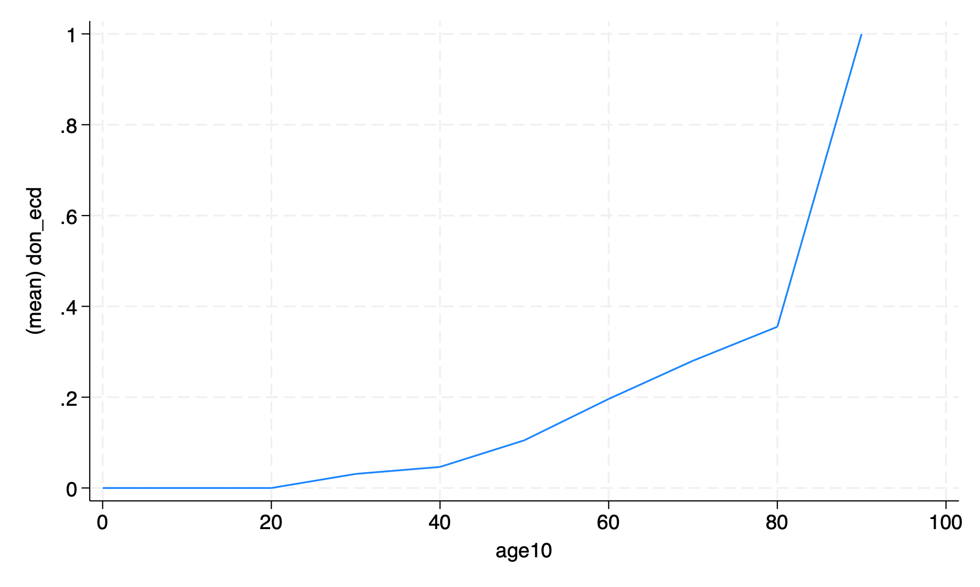
use "${repo}transplants", clear
gen age10 = round(age, 10)
     //one way to restore data after messing it up
     preserve 
         collapse (mean) don_ecd, by(age10)
         graph twoway line don_ecd age10
         graph export collpasebyage10.png,replace
     restore 
     count 
 

7. You have all your commands in your do file, right? Run your do file from the beginning and make sure your do file does exactly the same thing.