lab6 (including solutions)

lab6 (including solutions)#

data: transplants.dta donors_recipients.dta donors.dta

zoom: M T W Th F

stata18: updated color palatte

You’ll find that the content of chapter: twoway and lab6 complement each other!

Please use this lab as an opportunity to review the course material and prepare yourself for hw3. Sample responses to the lab questions are provided below.

Start Stata, open your do-file editor, write the header, and load transplants.dta.

use transplants, clear

Get a 10% random sample of the dataset. Specifically, follow these steps. (1) Set a seed number. (2) Generate a variable that includes a random number between 0 and 1 following a uniform distribution. An example was included in the first-ever .do file script you saw in this class from chapter: tokenize. (3) Sort by the random variable. (4) Keep the first 10% observations and drop the rest. (5) Drop the random variable.
```
count
set seed 2021
gen rdm=runiform()
sort rdm
keep if _n<=_N/10
drop rdm
count

//alternative
use transplants, clear
count
sample 10
count
```
Clear and reload transplants.dta.

use transplants, clear

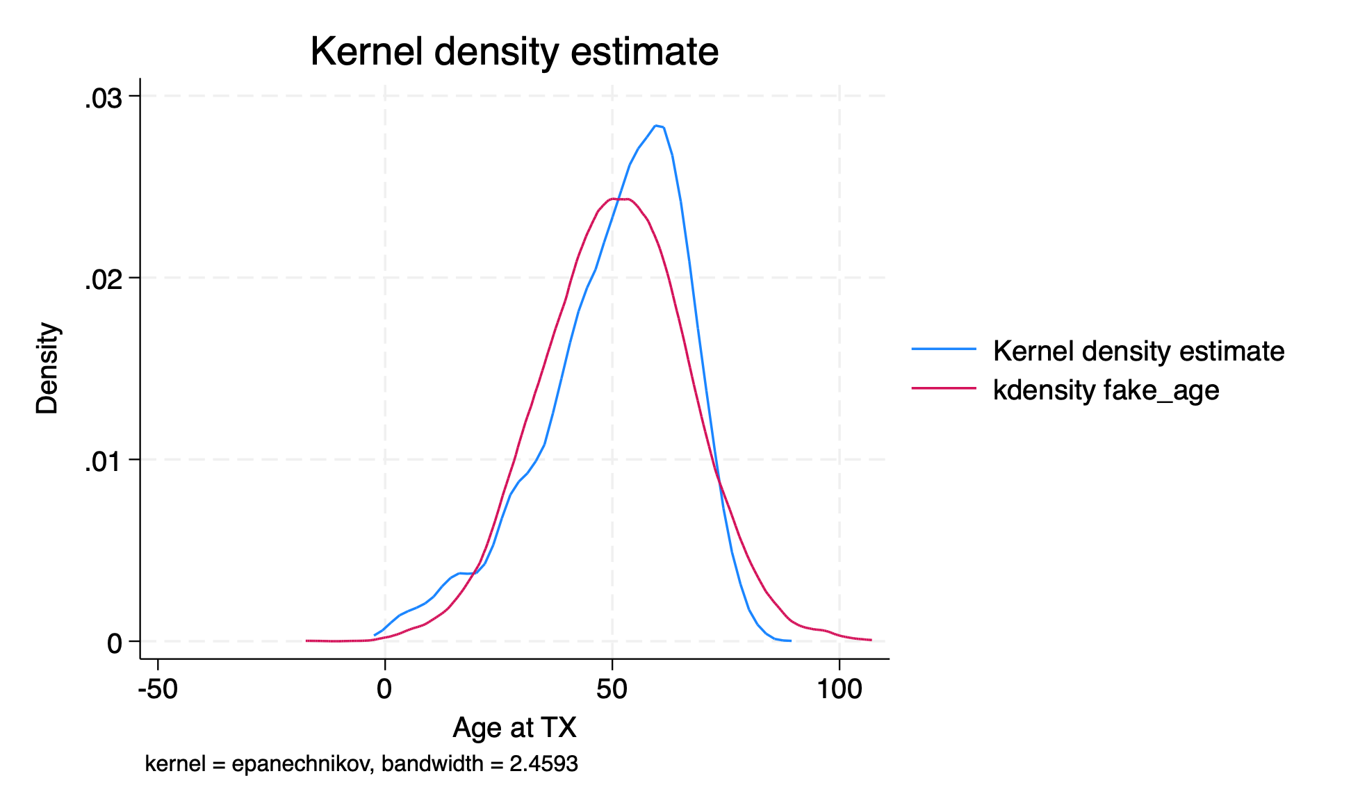
Generate a variable called fake_age which is a normally distributed random variable with mean and standard deviation equal to the mean and standard deviation of the actual age variable.

sum age
gen fake_age=rnormal(r(mean), r(sd))
sum age fake_age
compare age fake_age
kdensity age, addplot(kdensity fake_age)
list fake_id age fake_age in 1/10
graph export kdensity.png, replace 

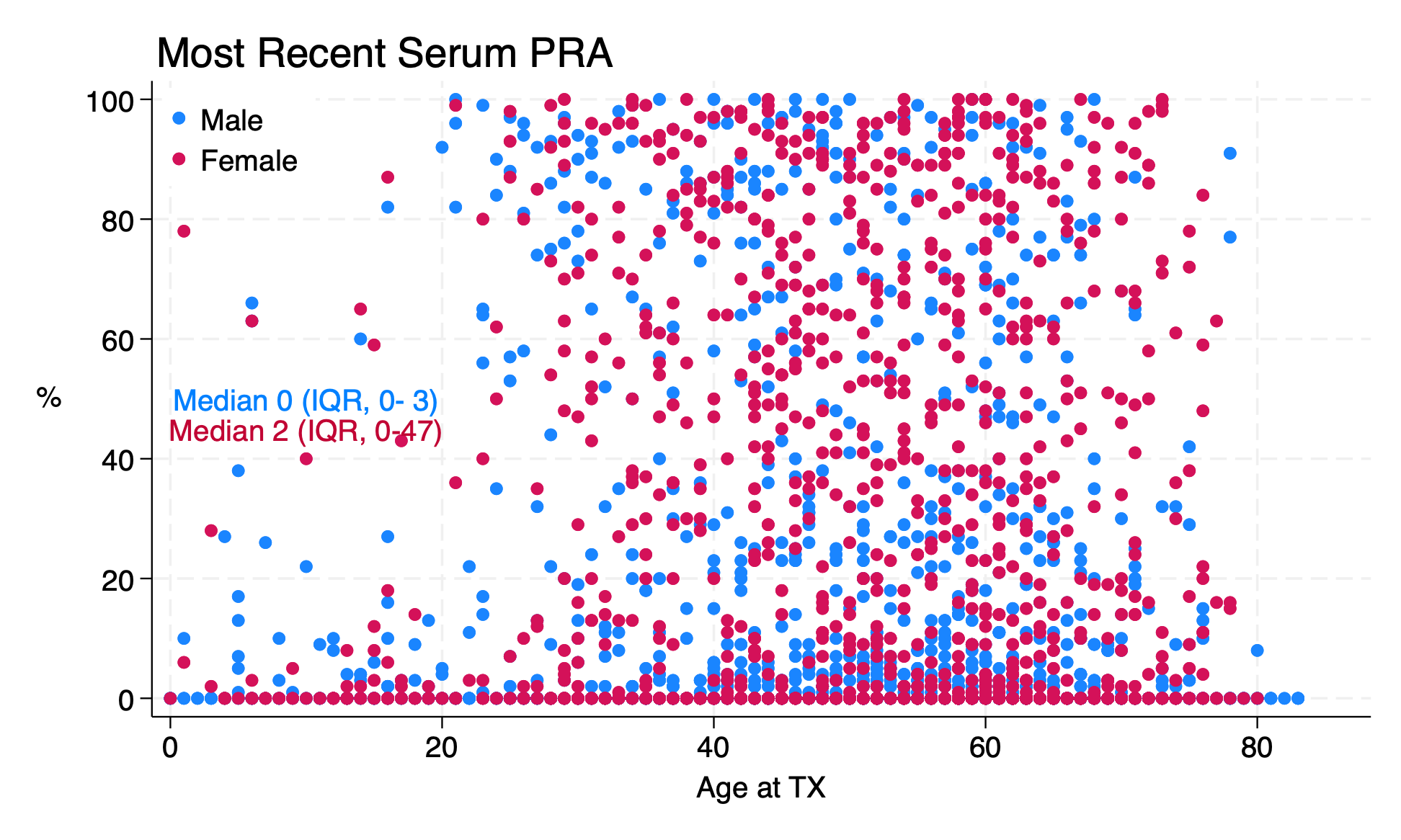
Make a scatter plot of peak PRA by age in transplant recipients. Does it look like there’s a relationship between peak PRA and age, and if so, what is the relationship?

   use transplants, clear 
   graph twoway scatter peak_pra age    //full syntax
   tw sc peak_pra age                 //abbreviated syntax
   
//explore other twoway options!!  
#delimit ;
forval f=0/1 { ;
	sum peak_pra if gender==`f', d ;
	local m_iqr_`f': di 
       "Median" %2.0f r(p50)
       " (IQR," %2.0f r(p25)
            "-" %2.0f r(p75)
            ")"
			;
} ;
tw (sc peak_pra age if gender==0)
   (sc peak_pra age if gender==1,
       legend(
           on
           ring(0)
           pos(11)
           lab(1 "Male")
           lab(2 "Female")
       )
       ti("Most Recent Serum PRA",pos(11))
       yti("%", orientation(horizontal))
   text(50 10 "`m_iqr_0'",col(midblue))
   text(45 10 "`m_iqr_1'",col(cranberry))
   )
   ;
   #delimit cr
   graph export lab6q5.png, replace 

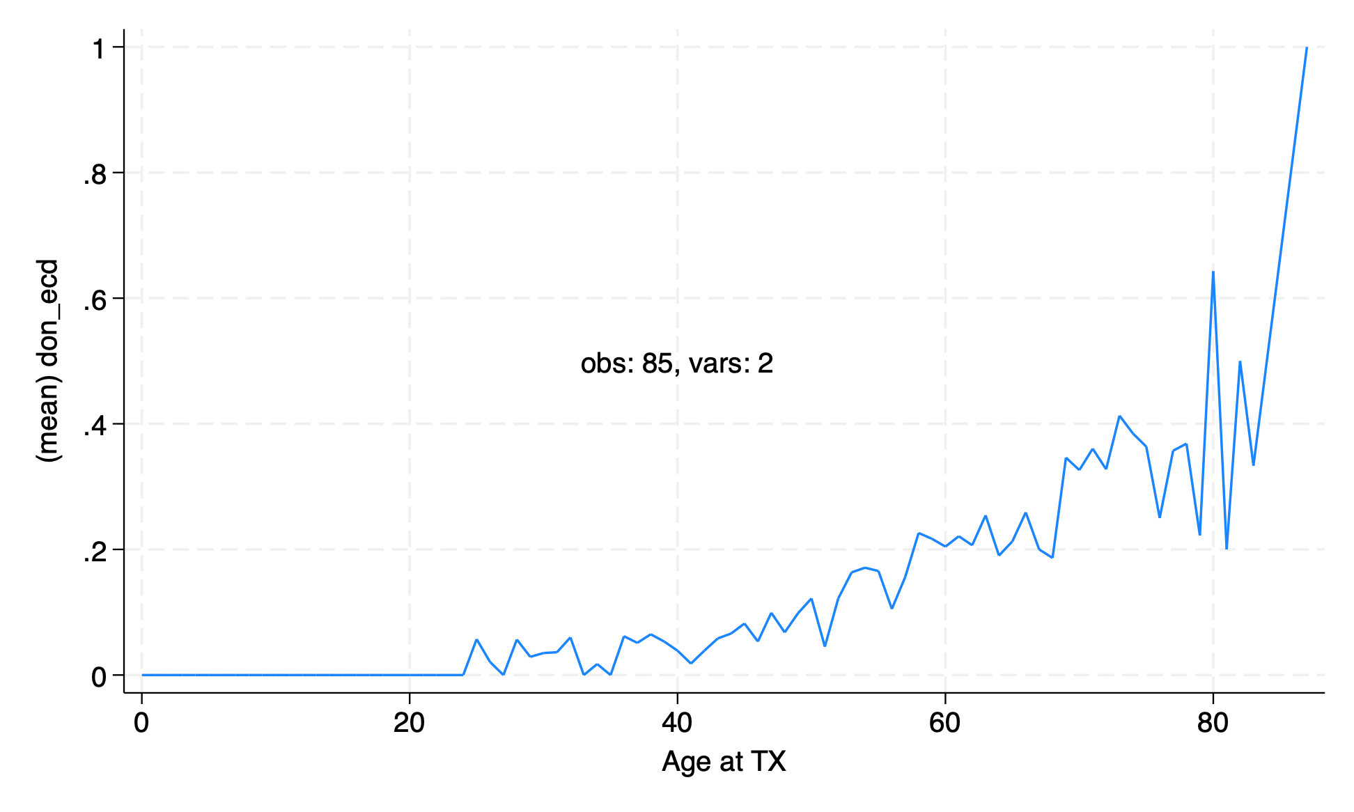
The graph of proportion of ECD transplants by age from the lecture was a little messy. Remake the graph with the age rounded to the nearest ten years.
- From the chapter: twoway

     use transplants, clear
     collapse (mean) don_ecd, by(age)
     graph twoway line don_ecd age, text(.5 40 "obs: `c(N)', vars: `c(k)'")
     graph export collpasebyage.png,replace
     count 
     
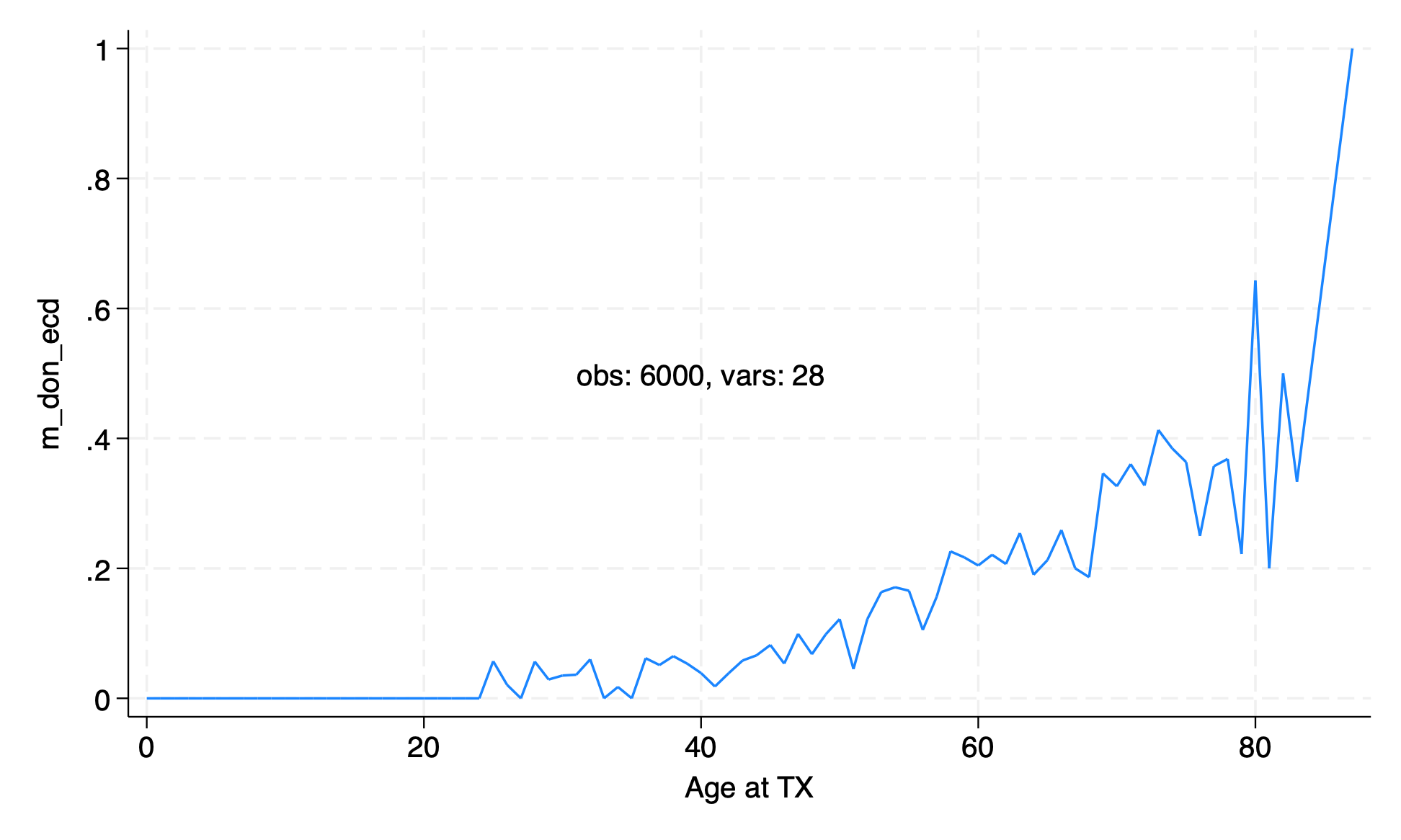
//alternative, without messing up the data
if c(N) == r(N) | c(N) == 6000 {
	
use transplants, clear
egen m_don_ecd=mean(don_ecd), by(age)
egen agetag=tag(age)
#delimit ;
line m_don_ecd age if agetag, 
    text(
    .5 40 
    "obs: `c(N)', vars: `c(k)'"
    ) 
    sort ;
#delimi cr
count
graph export lab6q6.png,replace 

}

After rounding

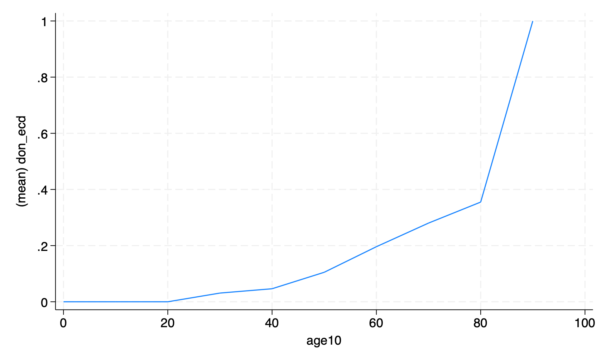
     use transplants, clear
     gen age10 = round(age, 10)
     //one way to restore data after messing it up
     preserve 
         collapse (mean) don_ecd, by(age10)
         graph twoway line don_ecd age10
         graph export collpasebyage10.png,replace
     restore 
     count 
 

You have all your commands in your do file, right? Run your do file from the beginning and make sure your do file does exactly the same thing. Also, in the spirit of hw1, and the spirit of the last 7 weeks, your .do file should look like this if you’ve adhered to the guidelines:

//you're welcome to flout
//   these guidelines after May 19
//but please don't flaunt your disregard 
//   for the didactic value before then

//collapse [-] at qui
qui {

//collapse [-] at if X {
qui {
	if 0 { //lab6 dofile
	if 1 { //transplants.dta
	if 2 { //runiform(),two methods
	if 3 { //transplants reload
	if 4 { //r(normal),kdensity
	if 5 { //embed macro in text then graph
	if 6 { //collpase & egen equivalence!!!!!!
	if 7 { //aesthetical .do file structure :)
       timer list  
       log close 
}

//alternative
//`if c(N) xxx {` merely placebolder
//but may become functional condition as 
//do file grows in complexity
//and accommodates more general stance
//e.g., due regard to c(os), c(version)
//or even to c(N), e(N), and r(N)
//suppose you have a rule of thumb:
//never to run a regression when c(N)<30?
//maybe ok to run, but not to report output when e(df)<30?
//well, maybe ok to do all above, but with a proviso in reported output?
//you are in position to incorporate any of the above into your .do files!!!

//collapse [-] at if `condition' {
qui {
    clear 
    cls
	if c(N) { //lab6 dofile
	if c(N)<1 { //transplants.dta
	if c(N)<2 { //runiform(),two methods
	if c(N)>3 { //transplants reload
	if c(N)>4 { //r(normal),kdensity
	if c(N)>5 { //embed macro in text then graph
	if c(N)>6 { //collpase & egen equivalence!!!!!!
	if c(N)==r(N) | c(N)==6000 { //aesthetical .do file structure 
       timer list  
       log close 
}