by#
video 04/13/2023 Includes introduction to program define
video 04/20/2023 Includes exercise in debugging & discussion of HW1
The figure below outlines a schema of what we covered last week and attempts to generalize it to several scenarios beyond what we might have time to cover in 5 weeks. For instance, you may replace sum with count, regression with kappa statistic estimation (as one of your classmates did), or yet still lincom with a matrix define m=r(table) step.
For the latter case, each matrix value will contain r() class macros, which you may capture and format in a local macro like so:
local b_age: di %3.1f m[1,4]
Where m is the matrix you defined and m[1,4] is the value in row1, column4. And here is a script that outputs r(table) following a Cox regression into an excel file:
Show code cell source
import networkx as nx
import matplotlib.pyplot as plt
#import numpy as np
#import sklearn as skl
#

#plt.figure(figsize=[2, 2])
G = nx.DiGraph()
#G.add_node(" ",  pos = (0, 3) )
G.add_node("regress",  pos = (1, 9.2) )
G.add_node("sum", pos = (-3, 4.5) )
G.add_node("lincom", pos = (1, 4.5) )
G.add_node("r()", pos = (-3, 0) )
G.add_node("r()*", pos = (1, 0) )
G.add_node("local", pos = (-1, -4.5))
G.add_node("embed", pos = (-1, -9))
G.add_edges_from([      ("regress", "lincom")])
G.add_edges_from([("sum", "r()"),     ("lincom", "r()*") ])
G.add_edges_from([("r()", "local"), ("r()*", "local")])
G.add_edges_from([("local","embed")])
nx.draw(G,
        nx.get_node_attributes(G, 'pos'),
        with_labels=True,
        font_weight='bold',
        node_size = 3500,
        node_color = "lightblue",
        linewidths = 3)
ax= plt.gca()
ax.collections[0].set_edgecolor("#000000")
ax.set_xlim([-10, 10])
ax.set_ylim([-10, 10])
plt.show()
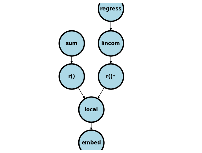
I’ve not illustrated where e() and c() fit in this scheme. But once you appreciate that r() values in memory can be revealed using return list, e() values using ereturn list, and c() values using creturn list then you will be set for life!!
The local macros you define will ultimately be embedded in programs you write or the text, tables, and figures of your final manuscripts.
We’ve seen how to embed a local macro in text after appropriately formatting the r() or e() content:
di "We have seen how to embed a `local macro' in text, but such macros may be embeded in tables and graphs as well!"
Remember:
names: r(), e(), c()
content: return, estimates, constants
these system-defined local macros may then be formatted to suit your needs in a user-defined local macro
In context of the first three weeks here is where things stand:
pwd—> dofile structure, working directory, location of outputr(mean)—> macros, local system-defined, user-definedby—> prelude toprogram define
For today’s session, by, you’ll use transplants.dta to demonstrate a few useful commands that we will put to good use over the coming weeks. You should be able to do most of this session on your own and at your convenience since it merely exposes you to various commands but not in the context of any specfic task.
use transplants, clear
What if we want a variable of the total number of records in each ABO blood type?
bys abo: gen cat_n = _N
So what did this code achieve?
tab cat_n
Let’s add labels to the groups:
#delimit ;
lab define abo_lab
   1 "A"
   2 "B"
   3 "AB"
   4 "O"
;
#delimit cr

lab values abo abo_lab
Now lets tabulate once again:
tab abo
Nice!
Ok. Do you remember these commands?
di c(N)

di c(k)
Lets create a disturbance to our setup to learn a few additional commands and their value to us:
qui do https://raw.githubusercontent.com/jhustata/book/main/sample-keep.ado
Is that a new command? Or are you already familiar with it? How about this:
samplekeep
What just happened?
di c(N)

di c(k)
Let’s rerun earlier commands to restore our sanity!
tab abo
Ok, then. It was a temporary disturbance and peace was restored!! We will talk more about the preserve and restore commands, often used together.
Back to the by command:
bys abo: egen age_byabo = mean(age)
Any idea what this command just achieved?
codebook age_byabo
What do you notice? Only four unique values! The egen command, like the gen command is used to define new variables in the dataset. However, the gen command applies values at the level of the individual. The egen command does so by group and yields summary statistics. To learn more type h egen.
qui regress peak_pra prev_ki
local coef_of_det: di %3.2f e(r2_a)*100

di "History of kidney transplant explains `coef_of_det'% of the variance in peak_pra."
From whence does e(r2_a) come? Where does it fit into our schema? (Hint: return list, ereturn list, creturn list)
//lets revisit this
regress age i.abo
lincom _b[3.abo]
What blood group has value 3?
return list
di %3.2f r(p)
di %3.2f r(estimate)
//does this output look familiar?
 lincom _cons + _b[3.abo]
 return list

//regression is a fancy way of estimating means for specified groups
 codebook age_byabo
Remember to use lincom appropriately, depending on what you wish to describe!
After a regression we may type ereturn list for all sorts of estimated values:
matrix define b = e(b)
matrix list b
di b[1,3]
You should explore the following commands, one-by-one, on your own:
tab rec_education, sum(age)
regress wait_yrs age, level(90)
count if age > 50
count if inrange(age,50,90)
list age dx rec_education in 1/5

//di c(N) " & " c(k)
use age dx using transplants, clear
use transplants in 1/50, clear
use transplants in 44
use transplants if rec_work==1
use a* p* using transplants in 1/100
//describe
describe, simple
describe, short
describe a*
describe using transplants.dta
describe r*, fullnames

//codebook
codebook
codebook rec_education rec_work abo
codebook a* e*, compact
codebook, problems

//list
list
list prev_ki wait_yrs if race==9
list *date in 1/10
list dx in 1/10, clean noobs
list age, fast

//count
count
count if rec_work==1
count if rec_work!=1
count if bmi<20 | bmi > 35
count if bmi>25 & bmi <30
count if !(age>18)
count if inrange(wait_yrs,4,6)
count if !inlist(gender,0,1)

//tabulate
tab abo
tab abo rec_hcv
tab gender, sum(age)
tab dx gender if age<40
tab dx gender,row
tab dx gender,col nofreq

tab dx gender, col nofreq chi2
return list

//summarize
sum
return list //not very useful; see schema above

sum age wait_yrs
return list //much more useful!

sum age wait_yrs, detail

//missingness
count if bmi > 30
count if bmi > 1000 //wha?
sum bmi //whats going on?
assert c(N) == r(N) //when do these diverge?
tab bmi if bmi > 1000
tab bmi if bmi > 1000, missing

count if bmi==.
count if bmi==.a
count if missing(bmi)
Let’s discuss missingness as its relevance emerges.
//manipulating data
gen age_lastyear=age-1
gen any_college=(rec_educ>=3)
g youngman=(age<40>)&(gender==0)
Variable types
byte: integer range -127 to 100
int: integer range -32767 to 32740
long: integer range \(\pm\) 2 billion
float: decimal, range \(\pm\) \(10^{38}\)
double: decimal, range \(\pm\) \(10^{307}\)
strings: e.g. str5 = string of length 5
You’ll need to specify the variable types as you start to right flexible programs with the program define command and syntax command with options such as, time(varname) event(varname) tmax(float)
If you wish to better understand these variables types, please explore those available to you in transplants.dta. Open the dataset and type desc.
use transplants, clear
describe
//generate
g byte young=(age<30>)
g age_f=age if gender==1
g age_spline=(age>40)*(age-40)

//_n and _N
g new_id=_n
gen total_records=_N
g percentile=100*_n/_N

//drop/keep
keep age gender bmi fake_id ra*
drop end_date

//remember: to load the original dataset again
use transplants, clear
keep in 1/100
drop if wait_yrs<1
keep if prev_ki==1
drop if age<18 & abo==2

//load data again
use transplants, clear
replace prev=0
replace wait_yrs=5 if wait_yrs>5
replace gender=gender+1
replace bmi=. if !inrange(bmi,17,50)

//rename
rename age age_at_transplant
rename gender female

use transplants, clear
rename (age gender)(age_at_transplant female)

//sort, gsort
list in 1/10
sort age
list in 1/10
sort age dx
list in 1/10
gsort -age dx -race
list in 1/10

//recode
recode rec_education (3 4 5 =9)
recode dx (1=1)(2=2)(*=9)
recode gender (0=1)(1=0),gen(male)

//display
sum wait_yrs
di "variable" _col(20) "mean"
di "wait time" _col(20) r(mean)

//capture
capture sum nonexistent_variable
capture di 4+3
capture di 4+

//assert
assert age<100
assert end_date>=transplant_date
assert inlist(gender,0,1)
assert 2<1
assert 0
assert c(edition_real)=="BE"
assert c(edition_real)=="MP"

//recode+label
#delimit ;
recode race
    (1=0 "Cauc")
    (2=1 "AA)
    (4=2 "Hisp/Latino")
    (5/9=3 "Other"),
        gen(race_cat)
;
#delimit cr

//preserve & restore
sum age

//indentation!
preserve
    drop if age<r(mean)
    sum age
restore

sum age
//comments

sum age //this displays mean, range, etc.

/*
Here's a long comment. It takes up several
lines, so I use the slash/asterisk.
*/

* Asterisk as first characater=comment

tab race * However, this doesn't work

if 0 { //background: ph.340.600

    1. we prefer `if 0 {' for comments
    2. and brief `//' annotations per `if int {' code-block
    3. do not use comments to explain a command
    4. that is what `help' is for
    5. our approach is avant-garde

}
Notebooks such as Jupyter notebook enable analysts to merge richer documentation together with analysis code, that isn’t quite possible in Stata. This class book is such an example of notebook that I have “hacked” from its Python roots for our Stata class.
For the curious few who looked closer at the schema outlined at the beginning of this class, you might have found some hidden but strange-looking code that produced the figure. That is python code.
I’m unable to input Stata code and display output in this Jupyter book. But the if integer { blocks that I’ve recommended for this class are actually inspired by Jupyter notebooks, where if 0 { represent documentation blocks and if int { represent code-blocks.
To me, if 0 { is infinitely more aesthetic than blocked-off green chuncks of annotated text, an approach familiar to most Stata users.
Jupyter books such as this are a major step forward in efforts toward reproducible research.
//line continuation

//Use `///` to make a Stata command span several lines in a .do file

recode race ///
    (1=1) ///
    (2=2) ///
    (4 5 6 7 9 = 9)

//That is the main-stream approach to line continuation. Ours?

#delimit ;
recode race
    (1=1)
    (2=2)
    (4 5 6 7 9)
;
#delimit cr
//labels
describe dx
label var dx "kidney disease diagnosis"

tab gender //is 1 male or female?
#delimit ;
label define g_label
    0 "0=Male"
    1 "1-Female"
;
#delimit cr
label values gender g_label
tab gender //much better
tab gender, nolabel //don't show label

//or?
g female=gender==1 //intuitive meaning of 1 & 0
//r-class examples
count if age < 45
di r(N) " young patients"

tab race abo, chi2
di "p-value: " r(p)
sum age
assert inrange(r(mean),45,55)

tab race abo, chi2
asset r(p) < 0.05
//display formats
sum bmi //command
local bmi_mean: di %4.1f r(mean) //r() -> local
di "Mean BMI: `bmi_mean' " //embed in text or other final output
//_b coefficient matrix

regress bmi gender age

#delimit ;
di "estimated BMI: " %3.2f _b[_cons] " + "
                     %3.2f _b[age] "*age (+ "
                           _b[gender] " if male)"
;
#delimit cr
//local macros
qui sum age if gender==0
local age_m: %3.1f r(mean)

qui sum age if gender==1
local age_f: %3.1f r(mean)

di "Mean age: `age_m' (males) `age_f' (females) "
//more local macros
local confounders age gender peak_pra
regress bmi wait_yrs `confoundres'
//program define
capture program drop table1
program define table1
    #delimit ;
    disp "Variable" _col(20) "mean (SD)"
                    _col(40) "range"
                    ;
    #delimit cr

    quietly sum age
    #delimit ;
    disp "age" _col(20) %3.2f r(mean)
              " (" %3.2f r(sd) ")"
               _col(40)  %3.2f r(min) "-" %3.2f r(max)
               ;
    #delimit cr
     //add more variables!
    end

    table1
//tagging
list abo gender spread
egen = tag
egen grouptag = tag(abo gender)
list abo gender spread if grouptag
use transplants, clear
egen ethtag = tag(ethcat)
bys ethcat: egen mean_bmi=mean(bmi) bys ethcat: egen mean_age=mean(age)
twoway scatter m~_bmi m~_age if ethtag
//conditionals
count if abo==1

if _N > 100 {

    di "Thats a big dataset

}

if _N > 10000 {

    di "That's a huge dataset"

}
//if and else
if _N > 10000 {

    di "That's a huge dataset"

}

else {

    di "Bah! Not so big."

}
//some `if` examples
quietly tab dx gender, chi2

if r(p) < 0.01 {

    di "p<0.01

}

else {

    di %3.2f r(p)
}
count if age<18
if r(N) >=200 {

    tab gender prev_ki, chi2

}

else {

    tab gender prev_ki, exact

}
count if !inlist(rec_hcv_antibody,0,1,.)

if r(N) ==0 {

    logistic rec_hcv_antibody age

}

else {

    di "Non-binary outcome."
    di "Can't do logistic regression"
}
//loops

forvalues i = 1/5 {

    di `i' //a local macro, given the notation!!

}
forvalues b = 35/45 {

    quietly count if age>=`b' & age<`b'+1
    disp "Age of `b': " r(N) " patients"

}