2. Return values, macros, programs#
Let’s briefly recap what we covered yesterday
Show code cell source
import networkx as nx
import matplotlib.pyplot as plt
#import numpy as np
#import sklearn as skl
#

#plt.figure(figsize=[2, 2])
G = nx.DiGraph()
G.add_node("user",  pos = (550,500) )
G.add_node("system",  pos = (-550,500) )
G.add_node("program",  pos = (-2000, 960) )
G.add_node("syntax",  pos = (2000, 950) )
G.add_node("ado", pos = (-3000, 550) )
G.add_node("do", pos = (3000, 550) )
G.add_node("command", pos = (-1900, 150) )
G.add_node("queue", pos = (1900, 150) )
G.add_node("results", pos = (0,0))
G.add_node("dta", pos = (0, -475))
G.add_node("log", pos = (-1900, -475))
G.add_node("excel", pos = (-4000, -475))
G.add_node("word", pos = (1900, -475))
G.add_node("html", pos = (4000, -475))
G.add_node("publish", pos = (0, -950))
G.add_edges_from([ ("program","ado"), ("syntax", "do")])
G.add_edges_from([("ado", "command"), ("do", "queue") ])
G.add_edges_from([("command", "results"), ("queue", "results"),("results","excel"),("results","word"),("results","html")])
G.add_edges_from([("results","dta"),("results","log")])
G.add_edges_from([("dta","publish"),("log","publish"),("excel","publish"),("word","publish"),("html","publish")])
nx.draw(G,
        nx.get_node_attributes(G, 'pos'),
        with_labels=True,
        font_weight='bold',
        node_size = 4500,
        node_color = "lightblue",
        linewidths = 3)
ax= plt.gca()
ax.collections[0].set_edgecolor("#000000")
ax.set_xlim([-5000, 5000])
ax.set_ylim([-1000, 1000])
plt.show()
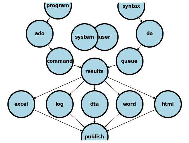
Results/Output
A sequence or queue of instructions
commands + syntax = codegiven to Stata via a do-file will generate resultsNever include results in your do-file when you share your work in this class and with future collaborators
Due diligence in the
open-scienceenterprise demands that othersreproduceyour results and findingsYour duty is to share only the
input, and ours is to reproduce youroutputso as to fullfil our shared CredoPlease share your do-files and any third-party ado-files, if at all your script or do-file relies on third-party programs
Display/Files
.xlsx
.log
.dta
.docx
2.1 xlsx#
use transplants, clear
putexcel set table1, replace
putexcel A1="Table 1. Demographic and clinical characteristics of kidney transplant recipients"
putexcel B1="N=`c(N)'"
2.2 log#
log using chi2.log, replace
use transplants
tab dx gender, row  chi2
. tab dx gender, row  chi2

+----------------+
Key
------------------
frequency
row percentage
+----------------+

Primary            gender
Diagnosis      |    0    |    1	    | Total
---------------+---------+----------+------
1=Glomerular   |  237    |    187   |	 424
               |  55.90  |   44.10  | 100.00
---------------+---------+----------+------
2=Diabetes     | 60      |  37	    | 97
               | 61.86   |  38.14   | 100.00
---------------+---------+----------+------
3=PKD          | 81      |  66	    | 147
               | 55.10   |  44.90   | 100.00
---------------+---------+----------+------
4=Hypertensive | 316     |  176	    | 492
               | 64.23   |  35.77   | 100.00
---------------+---------+----------+------
5=Renovascular | 24      |  15	    | 39
               | 61.54   |  38.46   | 100.00
---------------+---------+----------+------
6=Congenital   | 46      |  22	    | 68
               | 67.65   |  32.35   | 100.00
---------------+---------+----------+------
7=Tubulo       | 32      |  35	    | 67
               | 47.76   |  52.24   | 100.00
---------------+---------+----------+------
8=Neoplasm     | 8       |  5	    | 13
               | 61.54   |  38.46   | 100.00
---------------+---------+----------+------
9=Other        | 421     |  232	    | 653
               | 64.47   |  35.53   | 100.00
---------------+---------+----------+------
Total          | 1,225   |  775     | 2,000
               | 61.25   |  38.75   | 100.00

Pearson chi2(8) =  18.4805	Pr	= 0.018

.
If you review your log-file you’ll find results similar to those above. But these are not in the typical format seen in peer-reviewed work. For instance, p-values are usually reported in a format that depends on their exact value:
return list
qui {
    if r(p) < 0.01 {
	   local p: di "p < 0.01"
    }
    else if inrange(r(p),0.01,0.05) {
	   local p: di %3.2f r(p)
    }
    else {
	   local p: di %2.1f r(p)
    }
	noi di "p = `p'"
}
. return list

scalars:
r(N) =  2000
r(r) =  9
r(c) =  2
r(chi2) =  18.48047641017726
r(p) =  .0178990677414798

. qui {
p = 0.02
We’ll stop here for purposes of introducing the log-file as one of the file formats used to store output and results from analyes. Let’s close the file now.
log close
. log close
name:  <unnamed>
log:  /Users/d/Desktop/chi2.log
log type:  text
closed on:  20 Jun 2023, 05:46:13


--------------------------------------------------------------
2.3 dta#
cls
clear
postutil clear
postfile pp str80 a float(b c) using output.dta, replace
post pp ("1") (24.4) (123)
post pp ("2") (31.5) (164)
post pp ("3") (29.0) (118)
postclose pp

use output, clear
list
. clear

. postutil clear

. postfile pp str80 a float(b	c)	using	output.dta,	replace

. post pp ("1") (24.4) (123)

. post pp ("2") (31.5) (164)

. post pp ("3") (29.0) (118)

. postclose pp

.
. use output, clear

. list


    a      b     c
__________________
1.  1   24.4   123
2.  2   31.5   164
3.  3     29   118


.
end of do-file

.
2.4 docx#
We may embed Stata results in a .docx file in two very distinct ways:
putdocx
dyndoc
2.4.1. Putdocx#
putdocx begin (Tell Stata you want to create a Word doc)
putdocx text etc. (Define the contents of the Word doc you will create)
putdocx save (Actually create the Word doc and write it to disk)
putdocx clear
putdocx begin
putdocx paragraph
putdocx text ("How to embed Stata results in .docx")
putdocx paragraph
putdocx text ("Author, MD MPH")
putdocx paragraph
putdocx text ("Background. A user downloads and installs a system of program files, mostly ado-files, which form the foundation of most of the commands used in Stata Programming. Using those commands and additional syntax written out sequentially in a do-file, the user creates well-formed instruction to Stata called a do-file script. Once the user runs this script, results are generated and displayed in the results window, in a graph, or in a format (.xlsx, .log, .dta, .docx, .md, LaTeX, .html, etc). The .docx file format is of specific interest to us right now. To illustrate how this may be achieved in Stata, we hereby introduce the putdocx command.")
putdocx paragraph
putdocx text ("Methods. We created a do-file and populated it with this abstract using plain text. Results that might be numeric, string, alphanumeric, or formatted as macros are manually embeded in the text. We then saved this document using the file extension .do; however, any text file extension will work (.txt, .md, .do, etc). In the key analysis, Y = b0 + b1X, where Y is life expectancy at birth in years, the outcome or dependent variable; X is the country, the predictor or independent variable being tested.")
putdocx paragraph
putdocx text ("Results. We identified the newly created .html file in our folder and opened it to compare its format to this markdown file. And we saw all that we had made, and behold, it was very good. Ghastly macros in the original markdown language now appeared as neatly formatted results. There were 68 observations and 6 observations in the analyzed dataset. Average life expectancy of all countries, b0, was 72 years. Difference in life expectancy among adjacent countries, b1, showed no trend or pattern and was 0.002 year, essentially zero, and p=0.95")
putdocx paragraph
putdocx text ("Conclusion. In walking you through syntax, do-file creation, queued commands, generated results, through to embedding neatly formatted output in .html, we believe you now have a solid sense of all that Stata has to offer you. These ideas can be generalized to embedding results in .xlsx, .log, .dta, .docx, etc.")
putdocx save myfirst.docx, replace
Author, MD MPH
Background. A user downloads and installs a system of program files, mostly ado-files, which form the foundation of most of the commands used in Stata Programming. Using those commands and additional syntax written out sequentially in a do-file, the user creates well-formed instruction to Stata called a do- file script. Once the user runs this script, results are generated and displayed in the results window, in a graph, or in a format (.xlsx, .log, .dta, .docx, .md, LaTeX, .html, etc). The .docx file format is of specific interest to us right now. To illustrate how this may be achieved in Stata, we hereby introduce the putdocx command.
Methods. We created a do-file and populated it with this abstract using plain text. Results that might be numeric, string, alphanumeric, or formatted as macros are manually embeded in the text. We then saved this document using the file extension .do; however, any text file extension will work (.txt, .md, .do, etc). In the key analysis, Y = b0 + b1X, where Y is life expectancy at birth in years, the outcome or dependent variable; X is the country, the predictor or independent variable being tested.
Results. We identified the newly created .html file in our folder and opened it to compare its format to this markdown file. And we saw all that we had made, and behold, it was very good. Ghastly macros in the original markdown language now appeared as neatly formatted results. There were 68 observations and 6 observations in the analyzed dataset. Average life expectancy of all countries, b0, was 72 years. Difference in life expectancy among adjacent countries, b1, showed no trend or pattern and was 0.002 year, essentially zero, and p=0.95
Conclusion. In walking you through syntax, do-file creation, queued commands, generated results, through to embedding neatly formatted output in .html, we believe you now have a solid sense of all that Stata has to offer you. These ideas can be generalized to embedding results in .xlsx, .log, .dta, .docx, etc.
2.4.2. dyndoc#
Identical to the .html approach discussed in the next section
But has some caveats that we will discuss
Word documents are not able to render LaTeX format
Author, MD MPH#
Background:
A user downloads and installs a system of program files, mostly ado-files, which form the foundation of most of the commands
used in Stata Programming. Using those commands and additional syntax written out sequentially in a do-file, the user creates
well-formed instruction to Stata called a do-file script. Once the user runs this script, results are generated and displayed
in the results window, in a graph, or in a format (.xlsx, .log, .dta, .docx, .md, LaTeX, .html, etc). The .docx file format is of specific
interest since its the one of the most widely used word processors. To illustrate how this may be achieved in Stata, we hereby introduce the dyndoc
command.
Methods:
We created a do-file and populated it with this abstract using markdown language. Anything
in this document that is not ordinary text including <<dd_version: 2>>, <<dd_do:nooutput>>, <</dd_do>>, <<dd_display: c(N)>> is a
markup.
Results that might be numeric, string, alphanumeric, or formatted as macros are embeded at these markedup points. We then saved this
document using the file extension .do; however, any text file extension will work (.txt, .md, .do, etc). To the pwd where we saved
this text file, we added a cascading style sheet stmarkdown.css and header.txt to enhance the aesthetic of our .html file. Finally, we typed the
following command into the Stata command window: dyndoc filename.do, saving(filename.docx) replace. In the key analysis, \(Y = \beta_0 + \beta_1 X\), where \(Y\) is life expectancy at birth in years, the outcome or dependent variable; \(X\) is the country, the predictor or independent variable being tested.
. webuse lifeexp, clear
(Life expectancy, 1998)
. encode country, gen(Country)
. quietly sum lexp
. qui local lexp_mean: di %3.0f r(mean)
. quietly sum Country
. qui local Country_mean: di r(mean)
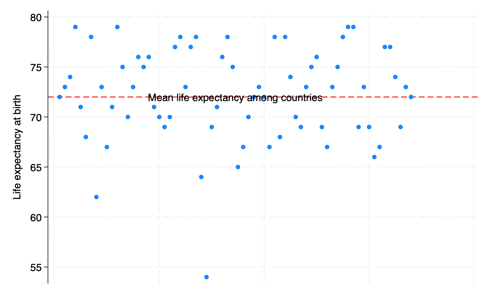
. twoway scatter lexp Country, ///
> xscale(off) ///
> yline(`lexp_mean', ///
> lc(red) ///
> lp(dash) ///
> ) ///
> text(`lexp_mean' `Country_mean' "Mean life expectancy among countries")
. graph export lexp_bycountry.png, replace
file /Users/d/Desktop/lexp_bycountry.png saved as PNG format
.
end of do-file
.
. qui {

.
. display c(N)
68

. display c(k)
6

. list in 1/5


    region	            country	    popgro~h	 lexp	    gnppc  safewa~r

1.  Europe & C. Asia	Albania	       1.2	        72	    810	    76
2.  Europe & C. Asia	Armenia	       1.1	        74	    460	    .
3.  Europe & C. Asia	Austria	       .4	        79	    26830   .
4.  Europe & C. Asia	Azerbaijan    1.4	        71	    480	    .
5.  Europe & C. Asia	Belarus	       .3	        68	    2180    .


.
end of do-file

.
Results: We identified the newly created .html file in our folder and opened it to compare its format to this markdown file. And we saw all that we had made, and behold, it was very good. Ghastly macros in the original markdown language now appeared as neatly formatted results. There were 68 observations and 6 observations in the analyzed dataset. Average life expectancy of all countries, \(\beta_0\), was 72 years. Difference in life expectancy among adjacent countries, \(\beta_1\), showed no trend or pattern and was 0.002 year, essentially \(zero\), and \(p = .95\)
Conclusions: In walking you through syntax, do-file creation, queued commands, generated results, through to embedding neatly formatted output in .html, we believe you now have a solid sense of all that Stata has to offer you. These ideas can be generalized to embedding results in .xlsx, .log, .dta, .docx, etc.
2.5 html#
2.5.1. How to embed Stata results in .html#
Author, MD MPH#
Background:
A user downloads and installs a system of program files, mostly ado-files, which form the foundation of most of the commands
used in Stata Programming. Using those commands and additional syntax written out sequentially in a do-file, the user creates
well-formed instruction to Stata called a do-file script. Once the user runs this script, results are generated and displayed
in the results window, in a graph, or in a format (.xlsx, .log, .dta, .docx, .md, LaTeX, .html, etc). The .html file format is of specific
interest since its the pathway to self-publication. To illustrate how this may be achieved in Stata, we hereby introduce the dyndoc
command.
Methods:
We created a do-file and populated it with this abstract using markdown language. Anything
in this document that is not ordinary text including <<dd_version: 2>>, <<dd_do:nooutput>>, <</dd_do>>, <<dd_display: c(N)>> is a
markup.
Results that might be numeric, string, alphanumeric, or formatted as macros are embeded at these markedup points. We then saved this
document using the file extension .do; however, any text file extension will work (.txt, .md, .do, etc). To the pwd where we saved
this text file, we added a cascading style sheet stmarkdown.css and header.txt to enhance the aesthetic of our .html file. Finally, we typed the
following command into the Stata command window: dyndoc filename.do, saving(filename.html) replace. In the key analysis, \(Y = \beta_0 + \beta_1 X\), where \(Y\) is life expectancy at birth in years, the outcome or dependent variable; \(X\) is the country, the predictor or independent variable being tested.
. webuse lifeexp, clear
(Life expectancy, 1998)

. encode country, gen(Country)

. quietly sum lexp

. qui local lexp_mean: di %3.0f r(mean)

. quietly sum Country

. qui local Country_mean: di r(mean)

. twoway scatter lexp Country, ///
>    xscale(off) ///
>    yline(`lexp_mean', ///
>       lc(red) ///
>       lp(dash) ///
>    ) ///
>    text(`lexp_mean' `Country_mean' "Mean life expectancy among countries")

. graph export lexp_bycountry.png, replace
file /Users/d/Desktop/lexp_bycountry.png saved as PNG format

.
end of do-file

.
. qui {

.
. display c(N)
68

. display c(k)
6

. list in 1/5


    region	            country	    popgro~h	 lexp	    gnppc  safewa~r

1.  Europe & C. Asia	Albania	       1.2	        72	    810	    76
2.  Europe & C. Asia	Armenia	       1.1	        74	    460	    .
3.  Europe & C. Asia	Austria	       .4	        79	    26830   .
4.  Europe & C. Asia	Azerbaijan    1.4	        71	    480	    .
5.  Europe & C. Asia	Belarus	       .3	        68	    2180    .


.
end of do-file

.
Results: We identified the newly created .html file in our folder and opened it to compare its format to this markdown file. And we saw all that we had made, and behold, it was very good. Ghastly macros in the original markdown language now appeared as neatly formatted results. There were 68 observations and 6 observations in the analyzed dataset. Average life expectancy of all countries, \(\beta_0\), was 72 years. Difference in life expectancy among adjacent countries, \(\beta_1\), showed no trend or pattern and was 0.002 year, essentially \(zero\), and \(p = .95\)
Conclusions: In walking you through syntax, do-file creation, queued commands, generated results, through to embedding neatly formatted output in .html, we believe you now have a solid sense of all that Stata has to offer you. These ideas can be generalized to embedding results in .xlsx, .log, .dta, .docx, etc.