1. Overview, commands, syntax#
Please respond to the brief entry survey that helps us better understand what your needs might be on day one. I’ll launch it on zoom for both the in-person and virtual attendees. The questions are listed here for your convenience. An identical exit survey will be launched on Friday to get a sense of what we’ve achieved over the five-day period.
How will you use Stata from 06/19/2023-06/23/2023?
Locally on my laptop
Remotely on another desktop or terminal
What operating system will you use locally or remotely?
MacOSX
Unix
Windows
Do you have any experience using Stata, SAS, R, Python, or any other statistical software?
No Experience. I have no prior experience with Stata and am unfamiliar with the software. Also, I have no experience with other statistical software such as SAS, R, Python, etc.
Basic Knowledge. I have a general understanding of basic commands but I require asistance to perform tasks.
Novice User. I am familiar with basic commands and can import data and do basic data cleaning. But I require guidance for more complex analyses.
Competent User. I am proficient in using Stata, SAS, R, Python, etc. for data exploration, descriptive statistics, basic inference (t-tests, chi-square tests), and regression
Advanced User. I can do multivariable regression and understand various statistical modeling options and techniques available in Stata, SAS, R, etc.
Expert User. I can write custom programs, macros, ado-files in Stata. Or I am an expert user of SAS, R, Python, etc. but have little to no experience with Stata.
1.1 Overview 🦀#
Ceci n’est pas une crabe
Show code cell source
import networkx as nx
import matplotlib.pyplot as plt
#import numpy as np
#import sklearn as skl
#

#plt.figure(figsize=[2, 2])
G = nx.DiGraph()
G.add_node("user",  pos = (550,500) )
G.add_node("system",  pos = (-550,500) )
G.add_node("program",  pos = (-2000, 960) )
G.add_node("syntax",  pos = (2000, 950) )
G.add_node("ado", pos = (-3000, 550) )
G.add_node("do", pos = (3000, 550) )
G.add_node("command", pos = (-1900, 150) )
G.add_node("queue", pos = (1900, 150) )
G.add_node("results", pos = (0,0))
G.add_node("dta", pos = (0, -475))
G.add_node("log", pos = (-1900, -475))
G.add_node("excel", pos = (-4000, -475))
G.add_node("word", pos = (1900, -475))
G.add_node("html", pos = (4000, -475))
G.add_node("publish", pos = (0, -950))
G.add_edges_from([ ("program","ado"), ("syntax", "do")])
G.add_edges_from([("ado", "command"), ("do", "queue") ])
G.add_edges_from([("command", "results"), ("queue", "results"),("results","excel"),("results","word"),("results","html")])
G.add_edges_from([("results","dta"),("results","log")])
G.add_edges_from([("dta","publish"),("log","publish"),("excel","publish"),("word","publish"),("html","publish")])
nx.draw(G,
        nx.get_node_attributes(G, 'pos'),
        with_labels=True,
        font_weight='bold',
        node_size = 4500,
        node_color = "lightblue",
        linewidths = 3)
ax= plt.gca()
ax.collections[0].set_edgecolor("#000000")
ax.set_xlim([-5000, 5000])
ax.set_ylim([-1000, 1000])
plt.show()
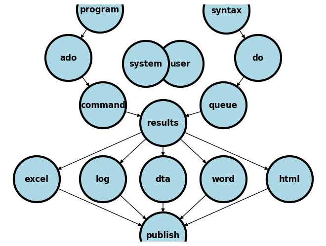
We are going to distinguish between two fundamental perspectives in this class:
System
Native (stata application, support files,
.adofiles)If you type
which helpinto your command window you get something like:/Applications/Stata/ado/base/h/help.ado
Third-party (typically
.adofiles)When I type
which table1_afecdviI get/Applications/Stata/ado/base/t/table1_afecdvi.ado
Your
.adofiles (you’ll learn to write & install your own programs)Since you don’t have
table1_afecdvi.adoinstalled you’ll getcommand table1_afecdv not found as either built-in or ado-file
User
Known
Instructor
Teaching assistants
Students
Collaborators
Unknown
Anticipate (emphathize with different kinds of users)
Share code (on GitHub, for instance)
Care (user-friendly, annotated code)
The system is the Stata application and its a simple noun. It is not STATA, which gives the impression of being an acronym. I presume you’ve all installed Stata onto your local machines. If not I presume you’ll be doing so very soon or you will be remotely accessing it. The user includes you, me, the teaching assistants, collaborators, or strangers.
As a user, you will or have already downloaded and installed a system of programs, mostly ado-files, which form the foundation of all the commands you will be using in Stata. These are the native Stata system files.
But soon you will begin to write your own Stata programs or .ado files and install them into the system folders (as I’ve done with table1_afecdvi.ado). Then, it will be helpful to think of your role as part of the system. In your new role as system, it will be helpful to anticipate the needs of the known and unknown future users of your program. This will call for empathy (anticipating user needs), sharing (your code with others), and caring (that its user-friendly).
Installation
Local
MacOSX
Unix
Windows
Remote
Desktop
Windows
Cluster
Unix/Terminal
Local
-
file
edit
view
data
graphics
statistics
user
window
command ⌘ 1
results ⌘ 2
history ⌘ 3
variables ⌘ 4
properties ⌘ 5
graph ⌘ 6
viewer ⌘ 7
editor ⌘ 8
do-file ⌘ 9
manager ⌘ 10
help
Command
The very first
validword you type into the command window or on a line of code in a do fileRendered blue in color if its a native Stata command (on my machine)
A third-party program/command appears white and may not work if you share your do file with others
Your collaborators, TAs, and instructors must be warned about the need to first install such third-party programs
Syntax
The arrangement of words after a Stata command
Create well-formed instructions in Stata (i.e., the syntax of Stata)
Other terms or synonyms include code, Stata code, code snippet.
Input
Menu (see above: a menu-driven task outputs command and syntax in the results window)
do files (Stata script with a sequence of commands; you can copy & paste some from the results window)
ado files (Stata script with a program or a series of programs for specific or general tasks)
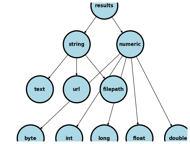
Output/Results
String
text (e.g.,
str49below = string of 49 characters including spaces)The median age in this population is 40 years old
url
https://www.stata-press.com/data/r8
filepath
/users/d/desktop
Numeric (types by range)
integer
byte: \(-127\) to \(100\)int: \(-32767\) to \(32740\)long: \(\pm 2\) billion
decimal
float: \(\pm 10^{38}\) billiondouble: \(\pm 10^{307}\) billion
-
Show code cell source
import networkx as nx
import matplotlib.pyplot as plt

#plt.figure(figsize=[2, 2])
G = nx.DiGraph()
G.add_node("results", pos = (500,960))
G.add_node("string", pos = (-1000, 400) )
G.add_node("numeric", pos = (1900, 400) )
G.add_node("text", pos = (-3000, -250) )
G.add_node("url", pos = (-1000, -250) )
G.add_node("filepath", pos = (1000, -250) )
G.add_node("long", pos = (500, -960))
G.add_node("int", pos = (-1400, -960))
G.add_node("byte", pos = (-3500, -960))
G.add_node("float", pos = (2400, -960))
G.add_node("double", pos = (4500, -960))
G.add_edges_from([ ("results","string")])
G.add_edges_from([("string", "text"),("string", "url") ,("string", "filepath")])
G.add_edges_from([("numeric","byte"),("numeric","float"),("numeric","double"),("numeric","int")])
G.add_edges_from([("numeric","long"),("results","numeric")])

nx.draw(G,
        nx.get_node_attributes(G, 'pos'),
        with_labels=True,
        font_weight='bold',
        node_size = 4500,
        node_color = "lightblue",
        linewidths = 3)
ax= plt.gca()
ax.collections[0].set_edgecolor("#000000")
ax.set_xlim([-5000, 5000])
ax.set_ylim([-1000, 1000])
plt.show()
Embed
Results window
Graph
File: excel, log, dta, word, html, etc.
Publish/Markup
Self (e.g., GitHub)
Journal (e.g. JAMA)
Commercial (e.g. Pfizer Ad)
Let’s use a simple example to illustrate some of the terms we’ve introduced:
Menu
file > example datasets > lifeexp.dta > use
sysuse lifeexp.dtawebuse lifeexp.dtause https://www.stata-press.com/data/r8/lifeexp.dta
do file
Importing data
Exploring data
Analyzing data
Outputing results
ado file
basis of Stata commands
etc.
1.2 Command#
Let’s instruct Stata to import some data:
webuse lifeexp, clear
. webuse lifeexp, clear
(Life expectancy, 1998)

.
The results window has some output informing us that we’ve imported Life expectancy data from 1998. Now let’s explore these imported data:
display c(N)
display c(k)
describe
. display c(N)
68

. display c(k)
6

. describe

Contains data from https://www.stata-press.com/data/r18/lifeexp.dta
Observations:            68                  Life expectancy, 1998
Variables:                6                  26 Mar 2022 09:40
(_dta has notes)

Variable      Storage   Display    Value
name            type    format     label      Variable label

region          byte    %16.0g     region     Region
country         str28   %28s                  Country
popgrowth       float   %9.0g               * Avg. annual % growth
lexp            byte    %9.0g               * Life expectancy at birth
gnppc           float   %9.0g               * GNP per capita
safewater       byte    %9.0g               * Safe water
* indicated variables have	notes

Sorted by:

.
By now you should be quick to point out that display is a command. To better understand what this command does, you can type help display in the command window. If you do so, you’ll learn the following:
[P] display	--	Display strings and values of scalar expressions
			(View complete PDF manual entry)
We’ve already discussed (see output above) string and numeric values as the two types of output we will be dealing with in Stata. So the display command displays, as it were, these values based on the specific syntax you provide
Output values will typically have two properties:
Name (e.g.
c(N)andc(k))Content (i.e., number of observations and number of variables)
Such values as we will learn tomorrow are called macros. In this given example, these are system-defined macros. And as you might have already guessed, there are also user-defined macros. More on this tomorrow!
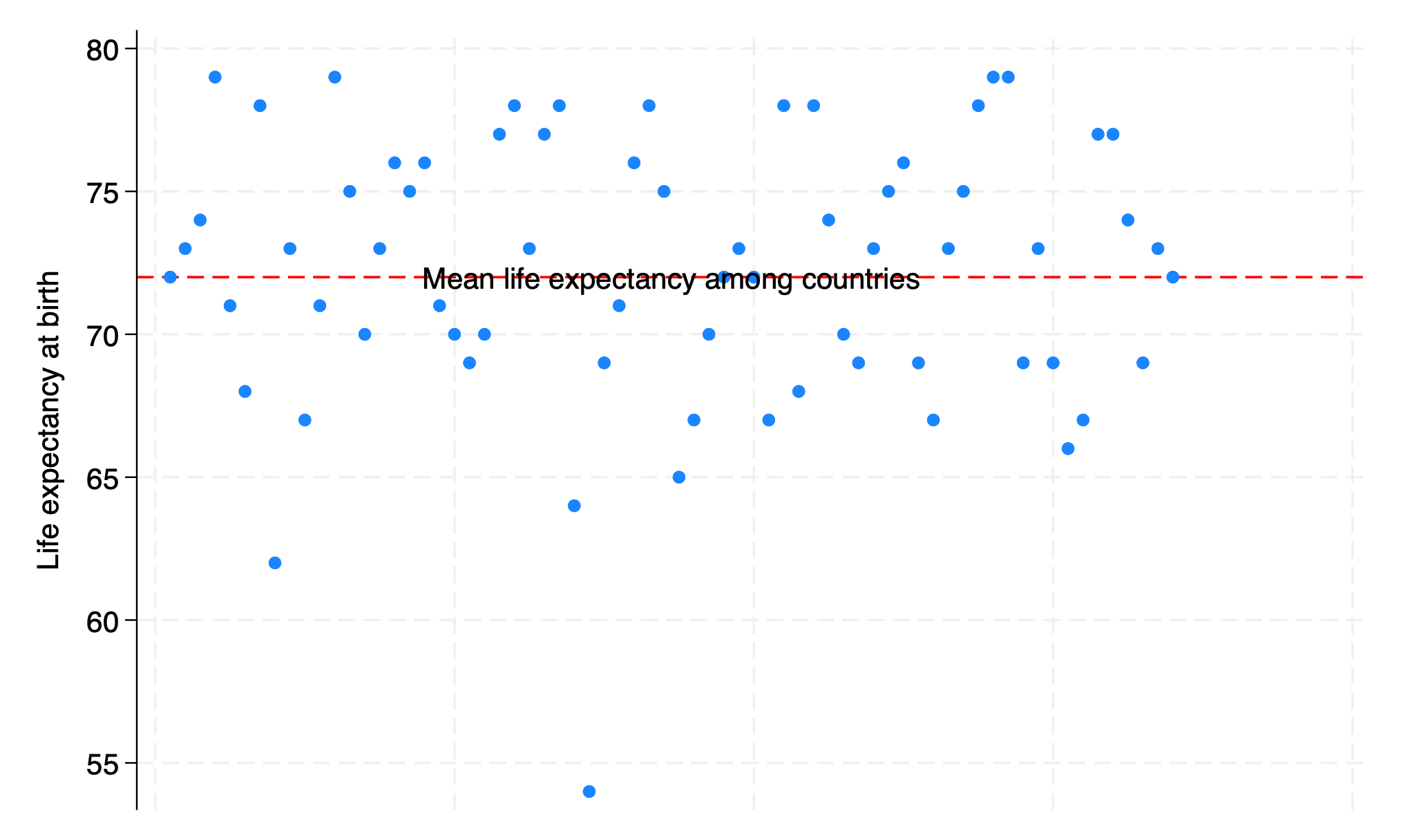
For now, let’s perform a basic analysis on our imported data to learn a little more about syntax and output:
webuse lifeexp, clear
encode country, gen(Country)
twoway scatter lexp Country, xscale(off)
graph export lexp_bycountry.png, replace
. webuse lifeexp, clear
(Life expectancy, 1998)

. encode country, gen(Country)

. twoway scatter lexp Country, xscale(off)

. graph export lexp_bycountry.png, replace
file /Users/d/Desktop/lexp_bycountry.png saved as PNG format

.
1.3 Syntax#
A few commands are useful on their own:
chelp
pwd
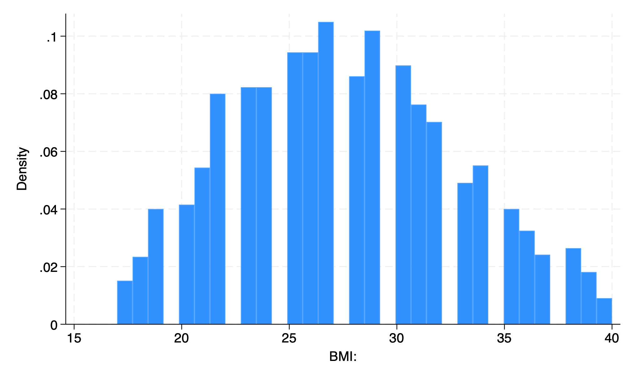
To name but a few. But the vast majority of commands will only work in context of the appropriate syntax. In this example below, the command clear is useful on its own. But set only becomes useful with additional syntax. Here we have obs 1000, instructing Stata to create an empty dataset with 1000 observations. The command generate with syntax bmi=rnormal(28,5) then instructs Stata to create a new variable bmi in a simulation of a random sampling process with replacement, 1000 times over, from a population with mean bmi of 28 and standard deviation of 5. Stata is then instructed to create a histogram of these simulated bmi sample and save the figure as a .PNG image. Hopefully this clarifies what a Stata command is and what syntax is. Together these make up Stata code.
 clear
 set obs 1000
 generate bmi=rnormal(28,5)
 histogram bmi, normal
 graph export bmi.png, replace
.  clear

.  set obs 1000
Number of observations (_N) was 0, now 1,000.

.  generate bmi=rnormal(28,5)

.  histogram bmi, normal
(bin=29, start=13.457429, width=.99248317)

.  graph export bmi.png, replace
file /Users/d/Desktop/bmi.png saved	as	PNG	format

.
end of do-file

.
In the above example the very first valid word is a command and is rendered blue on my machine but purple in this book. If you type any random word that has no corresponding ado-file, you’ll get an error message. Notice also that since its not a native Stata command, it appears black (or white), but not purple.
myfirstprogram
. myfirstprogram
command myfirstprogram is unrecognized
r(199);

.
The words that come after the command might be further commands or subcommands. If so, they’ll also be rendered blue on my machine. The ones that appear in white or black (dark or light mode) are either third-party programs/commands or they are part of the Stata syntax. By the end of tomorrow you’ll be writing your first program (which becomes a Stata command). And by Wednesday you’ll be adding requirements for syntax, which introduces user-defined input.