import matplotlib.pyplot as plt
import numpy as np
# Create data for the skill and challenge levels
skill_levels = np.linspace(0, 10, 100)
challenge_levels = np.linspace(0, 10, 100)
# Define the flow channel boundaries
flow_channel = skill_levels
# Adjust the phase and amplitude of the sinusoid wave
phase = np.pi / 16 # Reducing the wavelength by a quarter
amplitude = 1.5
flow_channel += np.sin(skill_levels + phase) * amplitude
# Define the yellow zone boundaries
yellow_zone_low = flow_channel - 1.5
yellow_zone_high = flow_channel + 1.5
# Define the sinusoid function with the middle yellow line as its axis
sinusoid = flow_channel + np.sin(skill_levels + phase) * amplitude
# Define the anxiety and boredom areas
anxiety_area = np.where(challenge_levels > flow_channel, challenge_levels, np.nan)
boredom_area = np.where(challenge_levels < flow_channel, challenge_levels, np.nan)
# Plotting
plt.figure(figsize=(8, 6))
# Plot the anxiety and boredom areas
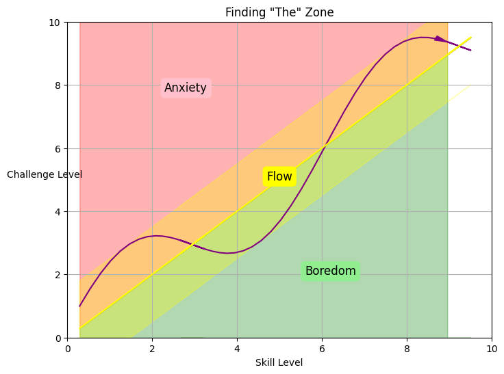
plt.fill_between(skill_levels, flow_channel, 10, color='red', alpha=0.3, label='Anxiety', interpolate=True)
plt.fill_between(skill_levels, 0, flow_channel, color='green', alpha=0.3, label='Boredom', interpolate=True)
plt.fill_between(skill_levels, yellow_zone_low, yellow_zone_high, color='yellow', alpha=0.3, label='Flow', interpolate=True)
# Plot the sinusoid function
plt.plot(skill_levels, sinusoid, color='purple', linestyle='-')
# Add arrowhead to the sinusoid line (flipped direction)
plt.arrow(skill_levels[-2], sinusoid[-2], skill_levels[-1] - skill_levels[-2], sinusoid[-1] - sinusoid[-2],
color='purple', length_includes_head=True, head_width=-0.15, head_length=-0.3)
# Plot the flow channel boundaries
plt.plot(skill_levels, flow_channel, color='yellow', linestyle='-')
# Set plot labels and title
plt.xlabel('Skill Level')
plt.ylabel('Challenge Level', rotation=0) # Rotate Y-axis label to be horizontal
plt.title('Finding "The" Zone')
# Set plot limits and grid
plt.xlim(0, 10)
plt.ylim(0, 10)
plt.grid(True)
# Set tick labels
tick_labels = ['0', '2', '4', '6', '8', '10']
plt.xticks(np.linspace(0, 10, 6), tick_labels)
plt.yticks(np.linspace(0, 10, 6), tick_labels)
# Add text annotations to label the areas
plt.text(2.8, 7.9, 'Anxiety', color='black', ha='center', va='center', fontsize=12, bbox=dict(facecolor='pink', edgecolor='pink', boxstyle='round'))
plt.text(5, 5.1, 'Flow', color='black', ha='center', va='center', fontsize=12, bbox=dict(facecolor='yellow', edgecolor='yellow', boxstyle='round'))
plt.text(6.2, 2.1, 'Boredom', color='black', ha='center', va='center', fontsize=12, bbox=dict(facecolor='lightgreen', edgecolor='lightgreen', boxstyle='round'))
# Display the plot
plt.show()